Nov 5, JDN 2458062

Continuing my series of blog posts on basic statistical concepts, today I’m going to talk about dummy variables. Dummy variables are quite simple, but for some reason a lot of people—even people with extensive statistical training—often have trouble understanding them. Perhaps people are simply overthinking matters, or making subtle errors that end up having large consequences.

A dummy variable (more formally a binary variable) is a variable that has only two states: “No”, usually represented 0, and “Yes”, usually represented 1. A dummy variable answers a single “Yes or no” question. They are most commonly used for categorical variables, answering questions like “Is the person’s race White?” and “Is the state California?”; but in fact almost any kind of data can be represented this way: We could represent income using a series of dummy variables like “Is your income greater than $50,000?” “Is your income greater than $51,000?” and so on. As long as the number of possible outcomes is finite—which, in practice, it always is—the data can be represented by some (possibly large) set of dummy variables. In fact, if your data set is large enough, representing numerical data with dummy variables can be a very good thing to do, as it allows you to account for nonlinear effects without assuming some specific functional form.
Most of the misunderstanding regarding dummy variables involves applying them in regressions and interpreting the results.
Probably the most common confusion is about what dummy variables to include. When you have a set of categories represented in your data (e.g. one for each US state), you want to include dummy variables for all but one of them. The most common mistake here is to try to include all of them, and end up with a regression that doesn’t make sense, or if you have a catchall category like “Other” (e.g. race is coded as “White/Black/Other”), leaving out that one and getting results with a nonsensical baseline.

You don’t have to leave one out if you only have one set of categories and you don’t include a constant in your regression; then the baseline will emerge automatically from the regression. But this is dangerous, as the interpretation of the coefficients is no longer quite so simple.

The thing to keep in mind is that a coefficient on a dummy variable is an effect of a change—so the coefficient on “White” is the effect of being White. In order to be an effect of a change, that change must be measured against some baseline. The dummy variable you exclude from the regression is the baseline—because the effect of changing to the baseline from the baseline is by definition zero.
Here’s a very simple example where all the regressions can be done by hand. Suppose you have a household with 1 human and 1 cat, and you want to know the effect of species on number of legs. (I mean, hopefully this is something you already know; but that makes it a good illustration.) In what follows, you can safely skip the matrix algebra; but I included it for any readers who want to see how these concepts play out mechanically in the math.
Your outcome variable Y is legs: The human has 2 and the cat has 4. We can write this as a matrix:

\[ Y = \begin{bmatrix} 2 \\ 4 \end{bmatrix} \]

What dummy variables should we choose? There are actually several options.

 

The simplest option is to include both a human variable and a cat variable, and no constant. Let’s put the human variable first. Then our human subject has a value of X₁ = [1 0] (“Yes” to human and “No” to cat) and our cat subject has a value of X₂ = [0 1].

This is very nice in this case, as it makes our matrix of independent variables simply an identity matrix:

\[ X = \begin{bmatrix} 1 & 0 \\ 0 & 1 \end{bmatrix} \]

This makes the calculations extremely nice, because transposing, multiplying, and inverting an identity matrix all just give us back an identity matrix. The standard OLS regression coefficient is B = (X’X)^-1 X’Y, which in this case just becomes Y itself.

\[ B = (X’X)^{-1} X’Y = Y = \begin{bmatrix} 2 \\ 4 \end{bmatrix} \]

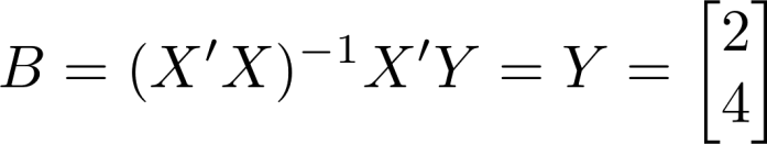
Our coefficients are 2 and 4. How would we interpret this? Pretty much what you’d think: The effect of being human is having 2 legs, while the effect of being a cat is having 4 legs. This amounts to choosing a baseline of nothing—the effect is compared to a hypothetical entity with no legs at all. And indeed this is what will happen more generally if you do a regression with a dummy for each category and no constant: The baseline will be a hypothetical entity with an outcome of zero on whatever your outcome variable is.
So far, so good.

But what if we had additional variables to include? Say we have both cats and humans with black hair and brown hair (and no other colors). If we now include the variables human, cat, black hair, brown hair, we won’t get the results we expect—in fact, we’ll get no result at all. The regression is mathematically impossible, regardless of how large a sample we have.

This is why it’s much safer to choose one of the categories as a baseline, and include that as a constant. We could pick either one; we just need to be clear about which one we chose.

Say we take human as the baseline. Then our variables are constant and cat. The variable constant is just 1 for every single individual. The variable cat is 0 for humans and 1 for cats.

Now our independent variable matrix looks like this:

\[ X = \begin{bmatrix} 1 & 0 \\ 1 & 1 \end{bmatrix} \]

The matrix algebra isn’t quite so nice this time:

\[ X’X = \begin{bmatrix} 1 & 1 \\ 0 & 1 \end{bmatrix} \begin{bmatrix} 1 & 0 \\ 1 & 1 \end{bmatrix} = \begin{bmatrix} 2 & 1 \\ 1 & 1 \end{bmatrix} \]

\[ (X’X)^{-1} = \begin{bmatrix} 1 & -1 \\ -1 & 2 \end{bmatrix} \]

\[ X’Y = \begin{bmatrix} 1 & 1 \\ 0 & 1 \end{bmatrix} \begin{bmatrix} 2 \\ 4 \end{bmatrix} = \begin{bmatrix} 6 \\ 4 \end{bmatrix} \]

\[ B = (X’X)^{-1} X’Y = \begin{bmatrix} 1 & -1 \\ -1 & 2 \end{bmatrix} \begin{bmatrix} 6 \\ 4 \end{bmatrix} = \begin{bmatrix} 2 \\ 2 \end{bmatrix} \]

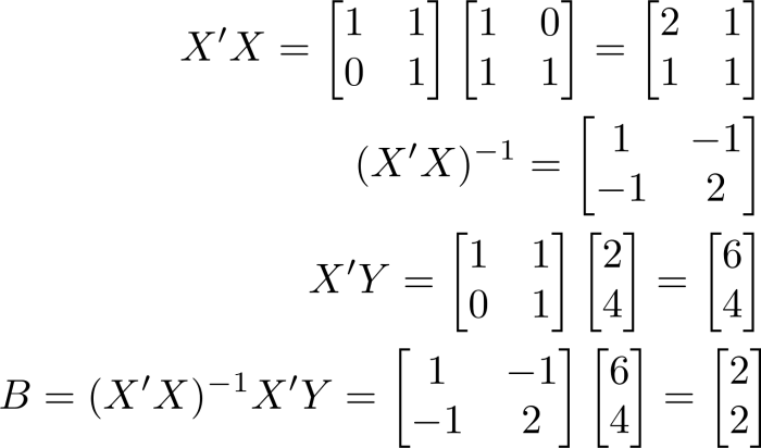
Our coefficients are now 2 and 2. Now, how do we interpret that result? We took human as the baseline, so what we are saying here is that the default is to have 2 legs, and then the effect of being a cat is to get 2 extra legs.
That sounds a bit anthropocentric—most animals are quadripeds, after all—so let’s try taking cat as the baseline instead. Now our variables are constant and human, and our independent variable matrix looks like this:

\[ X = \begin{bmatrix} 1 & 1 \\ 1 & 0 \end{bmatrix} \]

\[ X’X = \begin{bmatrix} 1 & 1 \\ 1 & 0 \end{bmatrix} \begin{bmatrix} 1 & 1 \\ 1 & 0 \end{bmatrix} = \begin{bmatrix} 2 & 1 \\ 1 & 1 \end{bmatrix} \]

\[ (X’X)^{-1} = \begin{bmatrix} 1 & -1 \\ -1 & 2 \end{bmatrix} \]

\[ X’Y = \begin{bmatrix} 1 & 1 \\ 1 & 0 \end{bmatrix} \begin{bmatrix} 2 \\ 4 \end{bmatrix} = \begin{bmatrix} 6 \\ 2 \end{bmatrix} \]

\[ B = \begin{bmatrix} 1 & -1 \\ -1 & 2 \end{bmatrix} \begin{bmatrix} 6 \\ 2 \end{bmatrix} = \begin{bmatrix} 4 \\ -2 \end{bmatrix} \]

Our coefficients are 4 and -2. This seems much more phylogenetically correct: The default number of legs is 4, and the effect of being human is to lose 2 legs.
All these regressions are really saying the same thing: Humans have 2 legs, cats have 4. And in this particular case, it’s simple and obvious. But once things start getting more complicated, people tend to make mistakes even on these very simple questions.

A common mistake would be to try to include a constant and both dummy variables: constant human cat. What happens if we try that? The matrix algebra gets particularly nasty, first of all:

\[ X = \begin{bmatrix} 1 & 1 & 0 \\ 1 & 0 & 1 \end{bmatrix} \]

\[ X’X = \begin{bmatrix} 1 & 1 \\ 1 & 0 \\ 0 & 1 \end{bmatrix} \begin{bmatrix} 1 & 1 & 0 \\ 1 & 0 & 1 \end{bmatrix} = \begin{bmatrix} 2 & 1 & 1 \\ 1 & 1 & 0 \\ 1 & 0 & 1 \end{bmatrix} \]

Our covariance matrix X’X is now 3×3, first of all. That means we have more coefficients than we have data points. But we could throw in another human and another cat to fix that problem.

 

More importantly, the covariance matrix is not invertible. Rows 2 and 3 add up together to equal row 1, so we have a singular matrix.

If you tried to run this regression, you’d get an error message about “perfect multicollinearity”. What this really means is you haven’t chosen a valid baseline. Your baseline isn’t human and it isn’t cat; and since you included a constant, it isn’t a baseline of nothing either. It’s… unspecified.

You actually can choose whatever baseline you want for this regression, by setting the constant term to whatever number you want. Set a constant of 0 and your baseline is nothing: you’ll get back the coefficients 0, 2 and 4. Set a constant of 2 and your baseline is human: you’ll get 2, 0 and 2. Set a constant of 4 and your baseline is cat: you’ll get 4, -2, 0. You can even choose something weird like 3 (you’ll get 3, -1, 1) or 7 (you’ll get 7, -5, -3) or -4 (you’ll get -4, 6, 8). You don’t even have to choose integers; you could pick -0.9 or 3.14159. As long as the constant plus the coefficient on human add to 2 and the constant plus the coefficient on cat add to 4, you’ll get a valid regression.
Again, this example seems pretty simple. But it’s an easy trap to fall into if you don’t think carefully about what variables you are including. If you are looking at effects on income and you have dummy variables on race, gender, schooling (e.g. no high school, high school diploma, some college, Bachelor’s, master’s, PhD), and what state a person lives in, it would be very tempting to just throw all those variables into a regression and see what comes out. But nothing is going to come out, because you haven’t specified a baseline. Your baseline isn’t even some hypothetical person with $0 income (which already doesn’t sound like a great choice); it’s just not a coherent baseline at all.

Generally the best thing to do (for the most precise estimates) is to choose the most common category in each set as the baseline. So for the US a good choice would be to set the baseline as White, female, high school diploma, California. Another common strategy when looking at discrimination specifically is to make the most privileged category the baseline, so we’d instead have White, male, PhD, and… Maryland, it turns out. Then we expect all our coefficients to be negative: Your income is generally lower if you are not White, not male, have less than a PhD, or live outside Maryland.

This is also important if you are interested in interactions: For example, the effect on your income of being Black in California is probably not the same as the effect of being Black in Mississippi. Then you’ll want to include terms like Black and Mississippi, which for dummy variables is the same thing as taking the Black variable and multiplying by the Mississippi variable.

But now you need to be especially clear about what your baseline is: If being White in California is your baseline, then the coefficient on Black is the effect of being Black in California, while the coefficient on Mississippi is the effect of being in Mississippi if you are White. The coefficient on Black and Mississippi is the effect of being Black in Mississippi, over and above the sum of the effects of being Black and the effect of being in Mississippi. If we saw a positive coefficient there, it wouldn’t mean that it’s good to be Black in Mississippi; it would simply mean that it’s not as bad as we might expect if we just summed the downsides of being Black with the downsides of being in Mississippi. And if we saw a negative coefficient there, it would mean that being Black in Mississippi is even worse than you would expect just from summing up the effects of being Black with the effects of being in Mississippi.

As long as you choose your baseline carefully and stick to it, interpreting regressions with dummy variables isn’t very hard. But so many people forget this step that they get very confused by the end, looking at a term like Black female Mississippi and seeing a positive coefficient, and thinking that must mean that life is good for Black women in Mississippi, when really all it means is the small mercy that being a Black woman in Mississippi isn’t quite as bad as you might think if you just added up the effect of being Black, plus the effect of being a woman, plus the effect of being Black and a woman, plus the effect of living in Mississippi, plus the effect of being Black in Mississippi, plus the effect of being a woman in Mississippi.