May 3 JDN 246164
I got into an argument a little while ago with an acquaintance of mine who is an avowed Marxist. He posted something that’s been going around Marxist social media about the “irony” that Marx’s labor theory of value is based on Smith and Ricardo’s labor theories of value (plural; they’re not the same), and thus when defenders of capitalism criticize the labor theory of value, they are in effect betraying their founding figures.
The first point I made in response to this was basically, “Yeah. So?” I think one thing that Marxists—at least this flavor of Marxist; I am prepared to exempt more serious Marxian economists—don’t really understand is that mainstream economists don’t have a founding figure that they worship and consider infallible. There is no inerrant text. I am fully prepared to acknowledge—and did, in fact, in that conversation, acknowledge—that Adam Smith made errors and his labor theory of value was one of them. And quite frankly, any defender of capitalism who worships Milton Friedman or Ayn Rand isn’t a mainstream economist, or is at best a very bad one.
My interlocutor then challenged me to describe these different labor theories of value, and I was foolish enough to take the bait, and then the whole conversation devolved into him playing this smug game of “That’s not what Marx really meant” and “clearly you haven’t read Das Kapital” (even though I have, but I admit it was several years ago; I did call up a PDF copy to refresh my memory during the conversation).
But it got me thinking about labor theories of value, and trying to understand why so many people find them seductive when it really doesn’t take much thought to show that they can’t possibly be right. (This post turned out to be a bit long, but I promise I won’t be as long-winded as Marx.)
So what’s wrong with labor theories of value?
If objects are valued based on the labor put into them, the following four propositions should hold:
- A project you spend 100 hours on which ultimately failed and produced nothing useful was extremely valuable.
- Everything in the Garden of Eden is worthless, because it doesn’t require labor to access.
- If you come up with a cure for cancer in a random stroke of insight, it’s worthless because you didn’t put any labor into it, even though both its utility (the lives it will save) and its price (the money you could make off of it) are surely astronomical.
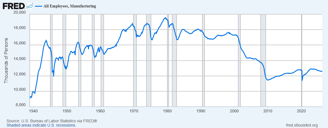
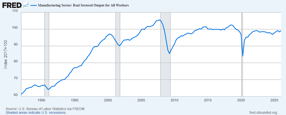
- Increased productivity is worthless, because all it does is make our goods worthless as we get better at making them.
All four of these propositions are clearly preposterous, and yet they all seem to follow directly from the basic concept of valuing things by the labor that goes into them. Mainstream economists eventually realized this, and gave up on labor theories of value in favor of the now-consensus utility theory of value.
To be fair, Marx was no idiot, and he did try to address concerns like these in Das Kapital. (Well, the first three he does; I’ll talk about the fourth one in a moment.) But the way he does so is by continually re-defining his terms in contradictory ways, so that by the time you get through the book, you realize he doesn’t even have a labor theory of value. He has many labor theories of value, and he substitutes them ad hoc whenever they seem to yield the conclusions he’s looking for.
For example: Sometimes he says that it’s the actual labor that goes in which matters. Other times that it’s the “usual” or “socially necessary” amount of labor. Other times that it’s the average amount of labor that would be required for this production across the whole economy. These are not the same thing! They yield radically different results in many cases!
Marx tries to distinguish use-value (approximately utility) from exchange-value (approximately price), which is good; those two things are different. It’s very important to distinguish price from value.
But then he doesn’t even use these concepts consistently! At one point, he gives us this absolute howler:
The use-value of the money-commodity becomes two-fold. In addition to its special use-value as
a commodity (gold, for instance, serving to stop teeth, to form the raw material of articles of
luxury, &c.), it acquires a formal use-value, originating in its specific social function.
– Das Kapital, Volume 1, Chapter 2, p. 63
No, dude. That is exchange-value. That is paradigmatic exchange-value. People mainly want gold because they can sell it at a high price to buy stuff that’s actually useful. If this is use-value, then the distinction between use-value and exchange-value collapses to, well, useless.
I think what Marx is doing here is that he wants use-value to always be higher than exchange-value, so that surplus-value can be the difference between them and always be positive. But gold is a very clear example of a good for which the price greatly exceeds the marginal utility, which I think you can convince yourself by imagining being stranded alone on a desert island with a crate full of gold. If that crate had contained non-perishable food, or water purification equipment, or tools and materials for building shelter, or best of all, a satellite phone and some solar panels, you’d be overjoyed to have it. Even a crate full of books, plushies, or underwear would have some use to you. (Plushies make better friends even than Wilson!) But gold? You have nothing to do but laugh—or cry—at the cruel irony. (And cash would be the same way, though maybe you could use the linen for something.)
But we actually do have a good explanation for how assets such as gold (and Bitcoin) can have prices far exceeding their marginal utility; expectations. If you expect that you’ll be able to sell an asset for more than you paid for it, you have reason to buy that asset, even if it’s useless to you. And for gold, that’s actually been a pretty smart gamble most of the time (Bitcoin, it very much depends on when you bought it). This could be a non-stationary equilibrium in rational expectations, or it could just be an ever-replenishing array of Greater Fools; but one way or another, the reason gold has a high price is that people expect it to have an even higher price in the future.
In fact, this seems like a deep flaw in capitalism! Marx could have spent a whole chapter on why gold is stupid and financial markets are basically a casino—he would have beaten out Keynes on that by decades. (If I were going to worship an economist, it would be Keynes. But again, I still don’t think his work is inerrant. Just very, very good.) But instead, Marx accepted that gold is priced the way it should be, and contorted his already-tortured theory of value into accommodating that.
I really don’t know why Marx was so insistent that all goods had to be valued based on labor. Marx actually had a lot of good insights about capitalism, and he wasn’t entirely wrong that capitalism as we know it breeds exploitation and ever-growing inequality. I believe that relatively simple reforms (like antitrust enforcement, co-ops, and progressive taxation) can solve, or at least mitigate, these problems, and allow us to enjoy the fruits of higher productivity that capitalism provides. But I recognize that I could be wrong about that; maybe some more radical change is genuinely needed. Yet this in no way vindicates Marx’s theory of value, which was simply wrongheaded from the start.
Indeed, why was he so insistent about it?
Why not simply give up on it, and adopt a new theory, or state it as an unsolved problem?
I have a hypothesis about that. Let me reprise proposition 4:
- Increased productivity is worthless, because all it does is make our goods worthless as we get better at making them.
This proposition is preposterous, as I’ve already said: A technology that allows you to make 100 cars with the same labor previously required to make 1 car does not make cars less useful. It simply makes them available to more people at lower prices, and this is generally a good thing.
But I think that Marx did not regard it as preposterous; in fact, I think he regarded it as true.
Consider this paragraph:
In proportion as capitalist production is developed in a country, in the same proportion do the
national intensity and productivity of labour there rise above the international level.2 The
different quantities of commodities of the same kind, produced in different countries in the same
working-time, have, therefore, unequal international values, which are expressed in different
prices, i.e., in sums of money varying according to international values. The relative value of
money will, therefore, be less in the nation with more developed capitalist mode of production
than in the nation with less developed. It follows, then, that the nominal wages, the equivalent of
labour-power expressed in money, will also be higher in the first nation than in the second; which
does not at all prove that this holds also for the real wages, i.e., for the means of subsistence
placed at the disposal of the labourer
– Das Kapital, Volume 1, chapter 22, p. 394
So he does get one qualitative fact right here: Nominal prices are higher in rich countries, for goods and services that are not traded across international borders. This is why we use purchasing power parity.
But he then goes on to say that real wages aren’t higher in rich countries. This… is just clearly false. By any reasonable measure, real wages are higher in the United States or France than they are in Congo or Haiti.
One can quibble with the particular measure used; I in fact happen to believe that we do overestimate real wages in the US by using the CPI instead of an index that better reflects the price of necessities. But there’s just no plausible way to say that a laborer in Malawi who makes $600 a year is at the same standard of living as a laborer in the US who makes $20,000. They might both be legitimately considered poor; but saying that real wages aren’t better here just isn’t plausible.
And Marx’s views on wages get weirder from there:
But hand-in-hand with the increasing productivity of labour, goes, as we have seen, the cheapening of the labourer, therefore a higher rate of surplus-value, even when the real wages are rising. The latter never rise proportionally to the productive power of labour. The same value in variable capital therefore sets in movement more labour-power, and, therefore, more labour.
Das Kapital, Volume 1, Chapter 24, p. 421
I’d in particular like to draw your attention to these two clauses: “the cheapening of the labourer, […] even when the real wages are rising.” What in the world does that mean? How can labor simultaneously get cheaper and more expensive? How can I be “cheapened” even as I am better off?
A bit later, he gets close to acknowledging that higher productivity increases value, but he characterizes it in a very strange way:
Labour transmits to its product the value of the means of production consumed by it. On the other
hand, the value and mass of the means of production set in motion by a given quantity of labour
increase as the labour becomes more productive. Though the same quantity of labour adds always
to its products only the same sum of new value, still the old capital value, transmitted by the
labour to the products, increases with the growing productivity of labour.
– Das Kapital, Volume 1, Chapter 24, p. 422
So what he seems to be saying here is that the value added from capital is itself denominated in terms of the labor that was used to create that capital. Yet this is a very strange accounting indeed, as I think a simple model will help you see.
Consider a productivity-enhancing technology.
Suppose that, initially, one can make 1 widget per person-hour. So, Marx says, the value of 1 widget is precisely 1 person-hour.
And suppose there are enough laborers to do 20 person-hours of work. Then we make 20 widgets, and we get value equal to 20 person-hours. Okay, seems reasonable so far.
Then, an engineer comes along, spending 100 hours to invent a machine that costs 10 person-hours to build, and can produce 1000 widgets using 10 person-hours of labor.
So the value of that machine, according to Marx as I understand him, is 10+X person-hours, where X is some amortized fraction of the 100 person-hours involved in inventing it. It’s unclear how to do this amortization; what time frame should be using? Once invented, the machine can be built many times. But I guess we could maybe make sense of it as the patent duration—the price of the machine will surely be higher during the time the patent is still valid, and I guess we could say that is somehow reflected in its value. (Notice how this is already getting pretty weird.)
Now, let’s go ahead and make 1000 widgets with the machine.
We have spent 10 person-hours of labor running the machine, another 10 building it, and we’re supposed to count in X from inventing it in the first place. X ranges somewhere between 0 and 100.
So at the low end, when X=0, these 1000 widgets have only cost us 20 person-hours to make, increasing productivity 50-fold. This is sort of where we expect to end up after the machine goes out of patent and becomes commonplace.
But at the high end, when X=100, these 1000 widgets have cost us 120 person-hours to make, increasing productivity a lesser, but still substantial, 8-fold. This might be where we find ourselves when the very first machine comes online and it’s still an experimental prototype.
Under the utility theory of value (which, again, virtually all mainstream economists, including both neoclassical, behavioral, and even Marxian economists, accept), the value of widgets has increased from U(20) to U(1000); exactly what this value is depends on how many consumers there are and what their utility functions are, but two things we can say for sure:
- This is definitely much higher than before. (Probably more than 10 but less than 50 times higher.)
- The value is the same regardless of how we account for the person-hours that went into inventing the machine.
- The cost gets lower over time, as the technology becomes established.
- Thus the value added should increase over time. (Whether or not profit does depends upon additional factors we haven’t modeled.)
But as Marx seems to be saying here (again, he may say differently elsewhere, but that’s kind of my point; he doesn’t have a coherent theory), we are to value these 1000 widgets as follows:
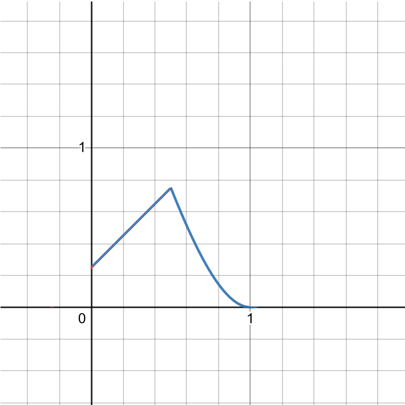
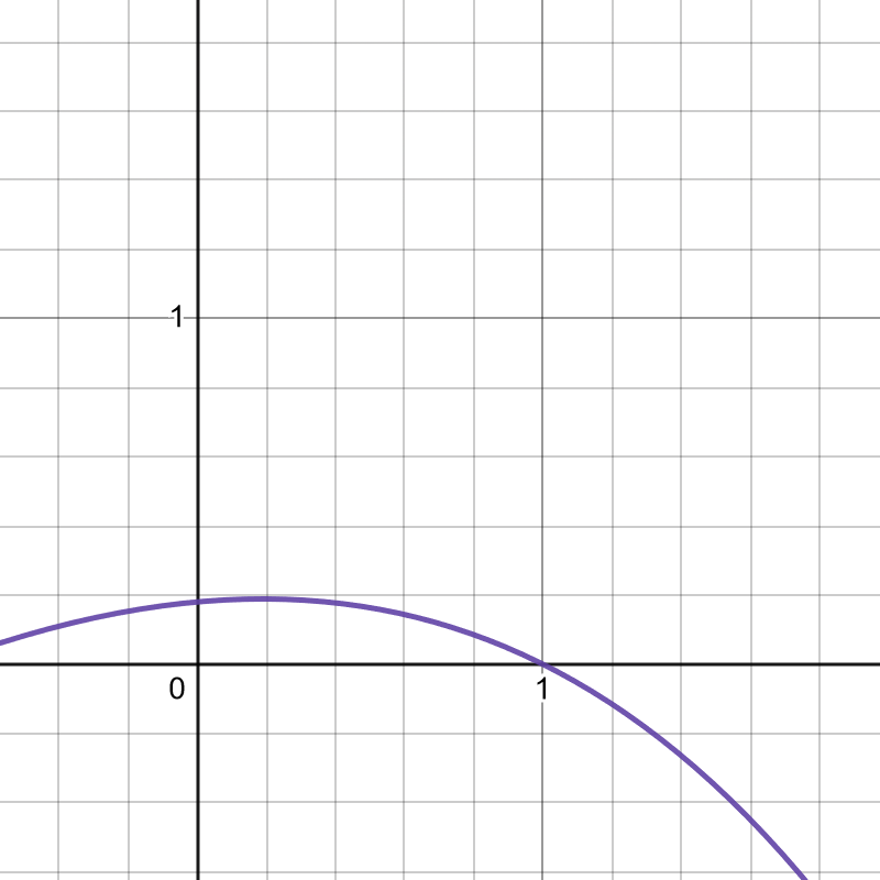
When the technology is new, X=100, and so the value of the 1000 widgets is 120 person-hours, the labor that went into inventing, producing, and using the machine. So this productivity enhancement has increased value somewhat—a 6-fold increase—but not all that much. And the value of each widget has been radically reduced: It is now only 0.12 person-hours, or about 7 person-minutes.
Yet once the technology becomes established, X=0, and so the value of the 1000 widgets is 20 person-hours, the labor that went into producing and using the machine. So now this productivity enhancement has not increased value at all. The value of each widget has fallen even further: It is now a mere 0.02 person-hours, or just over 1 person-minute.
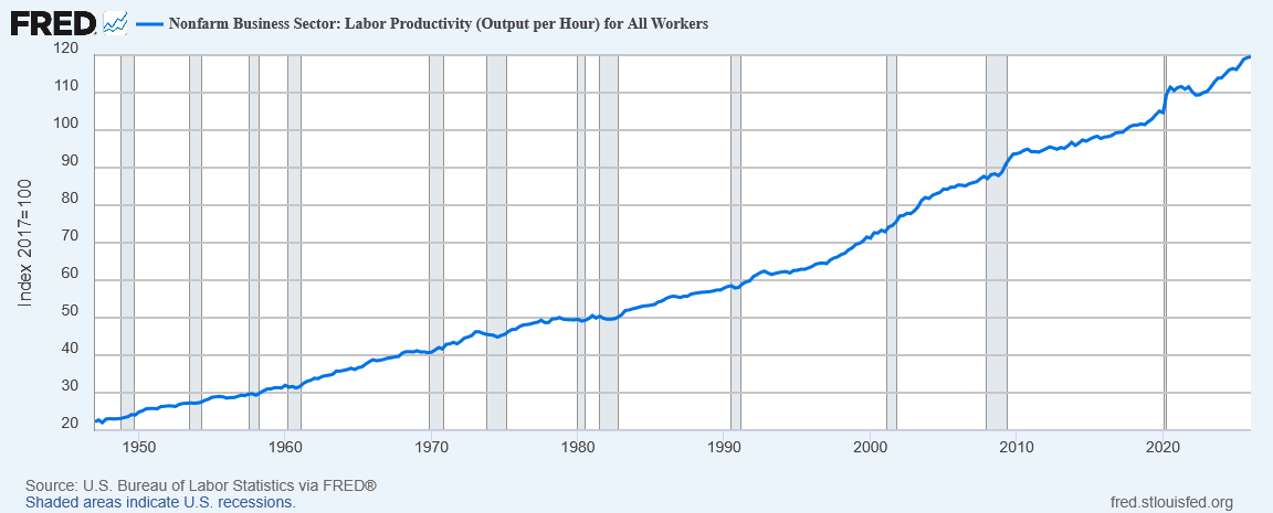
This weird dynamic, where technology increases value temporarily, then brings it back down to exactly what it was before, is clearly not how technology actually works. The value added from new technologies—in terms of utility, what really matters—is permanent and increasing over time.
Yet upon re-reading Marx and reflecting some more on his labor theories of value, I think Marx believed that this is actually what happens.
I think that Marx’s whole account of why the rate of profit must fall (even though it absolutely hasn’t, empirically, and even Marxian economists today recognize there’s no particular theoretical reason it should) is based on this misconception.
I think because he believed that labor is the correct measure of value, the fact that human beings can only do so much labor (which hasn’t really changed much over the millennia) means that standard of living can never really increase, because higher productivity simply translates into stuff becoming more and more worthless.
And I think part of where the confusion comes from is that price does sort of behave this way, at least qualitatively; no doubt in a world where widgets can be produced with only 1 minute of labor instead of 60 is one in which widgets are much cheaper to buy. But that doesn’t mean that their value has been correspondingly reduced; they are still just as useful (for whatever widgets do) as they were before, and any decline in marginal value merely comes from diminishing marginal utility as people get more and more of them.
Yet I think Marx didn’t want that result, because it seemed to imply that capitalism could actually make life better, even for workers. (As, empirically, it absolutely did.) He wanted to be able to prove that, despite all appearances, workers have gained absolutely nothing from capitalism and technology, and live just as poorly today as they did in the Middle Ages. And a labor theory of value was just the way to do that, for we only work slightly more hours today than most people did in the Middle Ages (and given the state of Medieval scholarship at the time, Marx may have even thought it was the same). Yet I for one am really a fan of vaccines and flush toilets; I don’t know about you.
He quickly realized many of the problems with this theory, and so he added more and more epicycles to try to correct these problems; but the result was a theory that wasn’t even coherent. Yet in part because of Marx’s incredibly dense and verbose writing style (please note; there are 547 pages in Volume I of Das Kapital, and it has three volumes.)it remained plausible enough to non-experts to catch on, and due to its very complexity, it becomes genuinely hard for anyone to understand. So then we can have the argument I had, where even as I clearly demonstrated the deep flaws in the theory, my interlocutor could always insist I hadn’t really understood what Marx was saying, and it was all my failing, not anything wrong with the theory, which is of course inerrant and handed down from On High.
For some people (not all, but some), Marxism really does seem more like a religion than a scientific theory: “I don’t know exactly what it means, but dammit, I know it’s true and you’ll never convince me otherwise.”
Is there a way to make a labor theory of value work?
I’m pretty well convinced that Marx’s labor theory of value is either wrong, or so incoherent as to be not even wrong. (Adam Smith’s and David Ricardo’s theories were coherent, so they were definitely just wrong.)
But could there, somewhere buried in all those hundreds of pages of mind-numbingly dense and self-contradictory text, be a theory worth salvaging?
Can I steelman the labor theory of value?
I’m going to give it a try.
Okay, so clearly it’s not the actual amount of labor used, as that runs afoul of proposition 1 immediately:
- A project you spend 100 hours on which ultimately failed and produced nothing useful was extremely valuable.
That’s nonsense, so we’ll rule that theory out.
Okay, maybe we can patch it up by saying it’s the socially necessary amount of labor required; the amount of labor that the most-efficient worker would require. Clearly, if you are spending 100 hours on something useless, you’re not being the most-efficient worker.
This seems to be closer to Marx’s account, but it still runs afoul of propositions 2, 3, and 4:
- Everything in the Garden of Eden is worthless, because it doesn’t require labor to access.
- If you come up with a cure for cancer in a random stroke of insight, it’s worthless because you didn’t put any labor into it, even though both its utility (the lives it will save) and its price (the money you could make off of it) are surely astronomical.
- Increased productivity is worthless, because all it does is make our goods worthless as we get better at making them.
Marx actually seemed to like proposition 4, but we can see that it’s wrong. So this is a problem.
Also, while propositions 2 and 3 may seem like extreme thought experiments, consider the following:
First, “The Garden of Eden” is very much what a Star Trek-style fully automated luxury communism would feel like. Many leftists say that they really would like to see such a world, and I agree with them on this. But on this theory of value, it’s all worthless, because nobody has to work to get anything.
Second, a sudden insight into a miracle cure that ends up becoming cheap and plentiful is pretty much what happened with penicillin and vaccines. Yes, there was some labor involved in making them (and still is), but it was clearly far less than the utility gained from all the improvements in health and lifespan that we have received from these inventions. Valuing these technologies in terms of their labor cost seems to completely miss the point of why they were such miracles.
So is there some other way to make a labor theory of value work?
The best I can come up with is this:
The value of a product is the amount of labor it would take to make that product by hand with pre-historic technology.
This is my attempt at steelmanning the labor theory of value. It does solve propositions 2, 3, and 4:
For 2, the fact that everything is handed to you (perhaps by robots) doesn’t change the fact that making it yourself would be really, really hard.
For 3, it’s much harder to make penicillin by hand than in a factory (though it can be done!), so improved penicillin technology is a gain in value. And every new vial of penicillin is worth the many hours that would have gone into making it by hand.
And for 4, any improvement in labor productivity works exactly how you’d expect: A machine that can do the work of 100 people produces 100 times as much value in goods. (In some ways, this is even more intuitive to most people than the utility theory of value, which predicts an increase, but not a one-to-one increase.)
So, okay, this theory is not preposterous, unlike everything we’ve considered so far.
But it really can’t be Marx’s theory, because he contradicts it very heavily in multiple places, and this theory, unlike his, does not predict that the rate of profit must fall. (Which, again, is good, because it doesn’t.)
Yet even this theory is ultimately unsatisfying, for the following reasons:
- Some products literally cannot be made by hand using pre-historic technology. Consider a graphics card or a strong-force microscope. In order to make these things, we had to make tools to make better tools to make even better tools to make still better tools to make yet even better tools to make staggeringly near-flawless tools to make them. Even if you had the complete schematics for all the necessary tools and machines, all the raw materials you needed, and an unlimited supply of labor, I’m not sure you could build a graphics card from scratch within a single lifetime.
- While it can account for the value of increased efficiency in producing a given good, it doesn’t seem to be able to account for the value of inventing whole new classes of goods. (Yes, penicillin can be made by hand using pre-historic tools, but nobody did as far as we know, and the value of that invention was absolutely enormous in a way that even this labor theory of value cannot account for.)
These two problems are related: The new products you can make now that you couldn’t before are made possible by a mix of new ideas and an accumulation of better and better tools.
As far as proposition 5, I think we might be able to shore up the theory by counting the value of capital accumulation in terms of the labor that would be needed at each level of technology: however many person-hours to make the optical microscope, and then however many person-hours to make lasers, and however many person-hours to make sulfuric acid, and so on and so forth, until you’ve finally added up all the labor that went into producing the things that produced the things that produced the things that produced the things that produced graphics cards.
But as for proposition 6? I think this is just fatal. I don’t think there’s any way for a labor theory of value to not systematically and catastrophically undervalue new discoveries and new inventions.
The whole point of new inventions is that they make new things possible or allow us to do things with far less effort or cost than before. The value they create is in the labor they save. But if they are things we theoretically could have done, just didn’t know how (like penicillin), then there is no value added by the discovery (though at least there can be a lot of value added by the actual production). And if they are things we couldn’t have done until we reached a certain level of technology and capital, the value added seems to all be captured by the production of each new tier of technology, with nothing left to go to the discovery itself.
Maybe there’s still a way to save this theory. But at some point, we have to stop and ask ourselves:
Why?
Why do we even want a labor theory of value, when we already have a utility theory of value?
Maybe it’s the fact that utility is hard to measure precisely, and so the idea of basing our value system on it is uncomfortable? Yet I think this is just a fact of life: The things that really matter are hard to measure precisely.
And it’s not as if we have absolutely no idea: We can tell the difference between happiness and suffering, and we can see how various products and technologies can contribute to happiness and alleviate suffering. (We can also see how some products and technologies can reduce happiness and contribute to suffering! Not all new technologies are good, and some products that are good for their users are bad for other people!)
Indeed, we even have a unit of measurement: The QALY. And for some particular technologies—such as penicillin and vaccines—we actually have a pretty good idea of the number of QALY they’ve added to the world, and it’s enormous.
I’m not even saying Marx was wrong about everything. He had some good ideas, actually. And Marxian economists today do sometimes come up with useful findings that can be integrated into a deeper understanding of political economy.
But he was wrong about some things, and the labor theory of value is one of them.