The role of innate activation in stochastic overload

Mar 26 JDN 2460030

Two posts ago I introduced my stochastic overload model, which offers an explanation for the Yerkes-Dodson effect by positing that additional stress increases sympathetic activation, which is useful up until the point where it starts risking an overload that forces systems to shut down and rest.

The central equation of the model is actually quite simple, expressed either as an expectation or as an integral:

Y = E[x + s | x + s < 1] P[x + s < 1]

Y = \int_{0}^{1-s} (x+s) dF(x)

The amount of output produced is the expected value of innate activation plus stress activation, times the probability that there is no overload. Increased stress raises this expectation value (the incentive effect), but also increases the probability of overload (the overload effect).

The model relies upon assuming that the brain starts with some innate level of activation that is partially random. Exactly what sort of Yerkes-Dodson curve you get from this model depends very much on what distribution this innate activation takes.

I’ve so far solved it for three types of distribution.

The simplest is a uniform distribution, where within a certain range, any level of activation is equally probable. The probability density function looks like this:

Assume the distribution has support between a and b, where a < b.

When b+s < 1, then overload is impossible, and only the incentive effect occurs; productivity increases linearly with stress.

The expected output is simply the expected value of a uniform distribution from a+s to b+s, which is:

E[x + s] = (a+b)/2+s

Then, once b+s > 1, overload risk begins to increase.

In this range, the probability of avoiding overload is:

P[x + s < 1] = F(1-s) = (1-s-a)/(b-a)

(Note that at b+s=1, this is exactly 1.)

The expected value of x+s in this range is:

E[x + s | x + s < 1] = (1-s)(1+s)/(2(b-a))

Multiplying these two together:

Y = [(1-s)(1+s)(1-s-a)]/[2(b-a)^2]

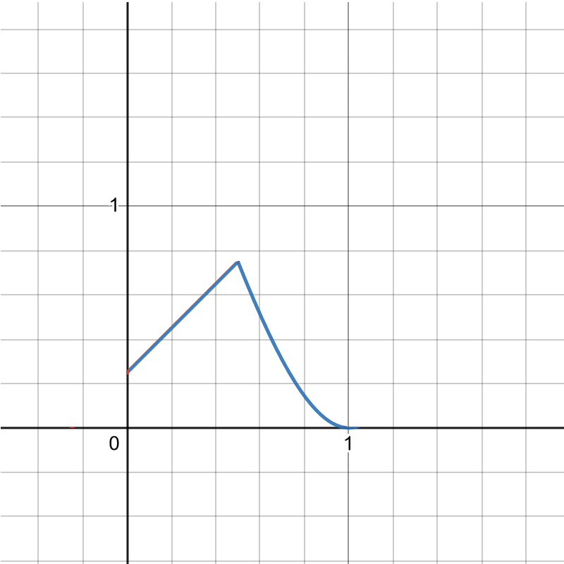
Here is what that looks like for a=0, b=1/2:

It does have the right qualitative features: increasing, then decreasing. But its sure looks weird, doesn’t it? It has this strange kinked shape.

So let’s consider some other distributions.

The next one I was able to solve it for is an exponential distribution, where the most probable activation is zero, and then higher activation always has lower probability than lower activation in an exponential decay:

For this it was actually easiest to do the integral directly (I did it by integrating by parts, but I’m sure you don’t care about all the mathematical steps):

Y = \int_{0}^{1-s} (x+s) dF(x)

Y = (1/λ+s) – (1/ λ + 1)e^(-λ(1-s))

The parameter λdecides how steeply your activation probability decays. Someone with low λ is relatively highly activated all the time, while someone with high λ is usually not highly activated; this seems like it might be related to the personality trait neuroticism.

Here are graphs of what the resulting Yerkes-Dodson curve looks like for several different values of λ:

λ = 0.5:

λ = 1:

λ = 2:

λ = 4:

λ = 8:

The λ = 0.5 person has high activation a lot of the time. They are actually fairly productive even without stress, but stress quickly overwhelms them. The λ = 8 person has low activation most of the time. They are not very productive without stress, but can also bear relatively high amounts of stress without overloading.

(The low-λ people also have overall lower peak productivity in this model, but that might not be true in reality, if λ is inversely correlated with some other attributes that are related to productivity.)

Neither uniform nor exponential has the nice bell-curve shape for innate activation we might have hoped for. There is another class of distributions, beta distributions, which do have this shape, and they are sort of tractable—you need something called an incomplete beta function, which isn’t an elementary function but it’s useful enough that most statistical packages include it.

Beta distributions have two parameters, α and β. They look like this:

Beta distributions are quite useful in Bayesian statistics; if you’re trying to estimate the probability of a random event that either succeeds or fails with a fixed probability (a Bernoulli process), and so far you have observed a successes and b failures, your best guess of its probability at each trial is a beta distribution with α = a+1 and β = b+1.

For beta distributions with parameters α and β, the result comes out to (I is that incomplete beta function I mentioned earlier):

Y = I(1-s, α+1, β) + I(1-s, α, β)

For whole number values of α andβ, the incomplete beta function can be computed by hand (though it is more work the larger they are); here’s an example with α = β = 2.

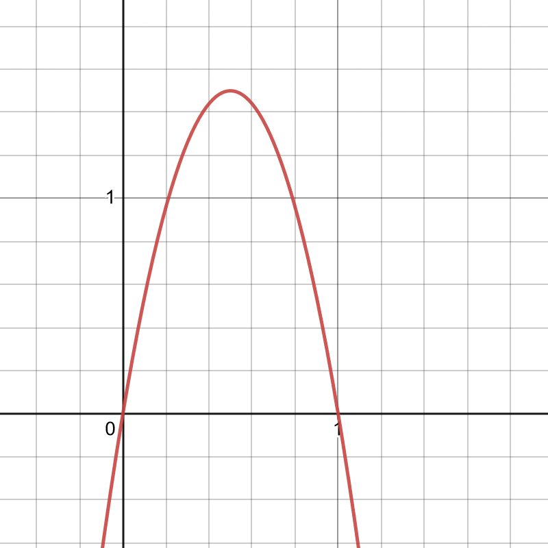
The innate activation probability looks like this:

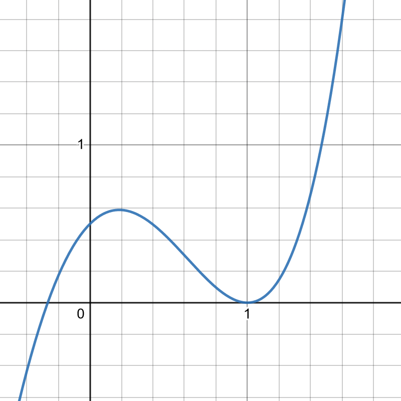
And the result comes out like this:

Y = 2(1-s)^3 – 3/2(1-s)^4 + 3s(1-s)^2 – 2s(1-s)^3

This person has pretty high innate activation most of the time, so stress very quickly overwhelms them. If I had chosen a much higher β, I could change that, making them less likely to be innately so activated.

These are the cases I’ve found to be relatively tractable so far. They all have the right qualitative pattern: Increasing stress increases productivity for awhile, then begins decreasing it once overload risk becomes too high. They also show a general pattern where people who are innately highly activated (neurotic?) are much more likely to overload and thus much more sensitive to stress.

The stochastic overload model

The stochastic overload model

Mar 12 JDN 2460016

The next few posts are going to be a bit different, a bit more advanced and technical than usual. This is because, for the first time in several months at least, I am actually working on what could be reasonably considered something like theoretical research.

I am writing it up in the form of blog posts, because actually writing a paper is still too stressful for me right now. This also forces me to articulate my ideas in a clearer and more readable way, rather than dive directly into a morass of equations. It also means that even if I do never actually get around to finishing a paper, the idea is out there, and maybe someone else could make use of it (and hopefully give me some of the credit).

I’ve written previously about the Yerkes-Dodson effect: On cognitively-demanding tasks, increased stress increases performance, but only to a point, after which it begins decreasing it again. The effect is well-documented, but the mechanism is poorly understood.

I am currently on the wrong side of the Yerkes-Dodson curve, which is why I’m too stressed to write this as a formal paper right now. But that also gave me some ideas about how it may work.

I have come up with a simple but powerful mathematical model that may provide a mechanism for the Yerkes-Dodson effect.

This model is clearly well within the realm of a behavioral economic model, but it is also closely tied to neuroscience and cognitive science.

I call it the stochastic overload model.

First, a metaphor: Consider an engine, which can run faster or slower. If you increase its RPMs, it will output more power, and provide more torque—but only up to a certain point. Eventually it hits a threshold where it will break down, or even break apart. In real engines, we often include safety systems that force the engine to shut down as it approaches such a threshold.

I believe that human brains function on a similar principle. Stress increases arousal, which activates a variety of processes via the sympathetic nervous system. This activation improves performance on both physical and cognitive tasks. But it has a downside; especially on cognitively demanding tasks which required sustained effort, I hypothesize that too much sympathetic activation can result in a kind of system overload, where your brain can no longer handle the stress and processes are forced to shut down.

This shutdown could be brief—a few seconds, or even a fraction of a second—or it could be prolonged—hours or days. That might depend on just how severe the stress is, or how much of your brain it requires, or how prolonged it is. For purposes of the model, this isn’t vital. It’s probably easiest to imagine it being a relatively brief, localized shutdown of a particular neural pathway. Then, your performance in a task is summed up over many such pathways over a longer period of time, and by the law of large numbers your overall performance is essentially the average performance of all your brain systems.

That’s the “overload” part of the model. Now for the “stochastic” part.

Let’s say that, in the absence of stress, your brain has a certain innate level of sympathetic activation, which varies over time in an essentially chaotic, unpredictable—stochastic—sort of way. It is never really completely deactivated, and may even have some chance of randomly overloading itself even without outside input. (Actually, a potential role in the model for the personality trait neuroticism is an innate tendency toward higher levels of sympathetic activation in the absence of outside stress.)

Let’s say that this innate activation is x, which follows some kind of known random distribution F(x).

For simplicity, let’s also say that added stress s adds linearly to your level of sympathetic activation, so your overall level of activation is x + s.

For simplicity, let’s say that activation ranges between 0 and 1, where 0 is no activation at all and 1 is the maximum possible activation and triggers overload.

I’m assuming that if a pathway shuts down from overload, it doesn’t contribute at all to performance on the task. (You can assume it’s only reduced performance, but this adds complexity without any qualitative change.)

Since sympathetic activation improves performance, but can result in overload, your overall expected performance in a given task can be computed as the product of two terms:

[expected value of x + s, provided overload does not occur] * [probability overload does not occur]

E[x + s | x + s < 1] P[x + s < 1]

The first term can be thought of as the incentive effect: Higher stress promotes more activation and thus better performance.

The second term can be thought of as the overload effect: Higher stress also increases the risk that activation will exceed the threshold and force shutdown.

This equation actually turns out to have a remarkably elegant form as an integral (and here’s where I get especially technical and mathematical):

\int_{0}^{1-s} (x+s) dF(x)

The integral subsumes both the incentive effect and the overload effect into one term; you can also think of the +s in the integrand as the incentive effect and the 1-s in the limit of integration as the overload effect.

For the uninitated, this is probably just Greek. So let me show you some pictures to help with your intuition. These are all freehand sketches, so let me apologize in advance for my limited drawing skills. Think of this as like Arthur Laffer’s famous cocktail napkin.

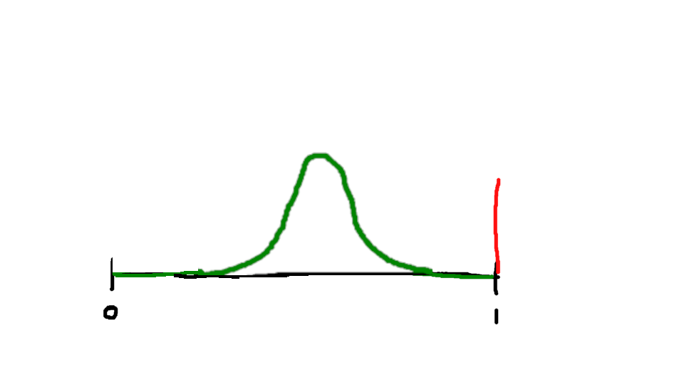
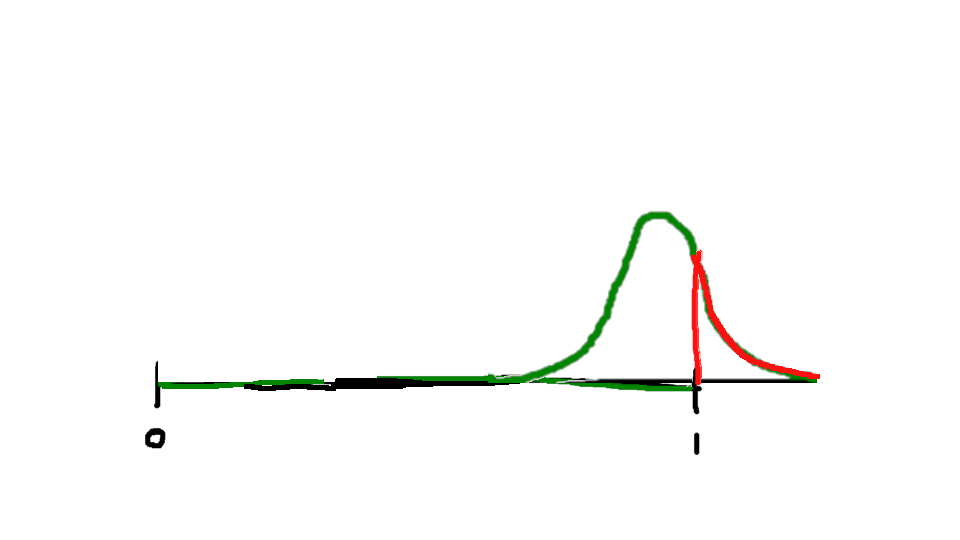
Suppose that, in the absence of outside stress, your innate activation follows a distribution like this (this could be a normal or logit PDF; as I’ll talk about next week, logit is far more tractable):

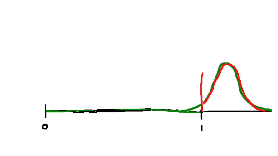
As I start adding stress, this shifts the distribution upward, toward increased activation:

Initially, this will improve average performance.

But at some point, increased stress actually becomes harmful, as it increases the probability of overload.

And eventually, the probability of overload becomes so high that performance becomes worse than it was with no stress at all:

The result is that overall performance, as a function of stress, looks like an inverted U-shaped curve—the Yerkes-Dodson curve:

The precise shape of this curve depends on the distribution that we use for the innate activation, which I will save for next week’s post.

On the quality of matches

Apr 11 JDN 2459316

Many situations in the real world involve matching people to other people: Dating, job hunting, college admissions, publishing, organ donation.

Alvin Roth won his Nobel Prize for his work on matching algorithms. I have nothing to contribute to improving his algorithm; what baffles me is that we don’t use it more often. It would probably feel too impersonal to use it for dating; but why don’t we use it for job hunting or college admissions? (We do use it for organ donation, and that has saved thousands of lives.)

In this post I will be looking at matching in a somewhat different way. Using a simple model, I’m going to illustrate some of the reasons why it is so painful and frustrating to try to match and keep getting rejected.

Suppose we have two sets of people on either side of a matching market: X and Y. I’ll denote an arbitrarily chosen person in X as x, and an arbitrarily chosen person in Y as y. There’s no reason the two sets can’t have overlap or even be the same set, but making them different sets makes the model as general as possible.

Each person in X wants to match with a person in Y, and vice-versa. But they don’t merely want to accept any possible match; they have preferences over which matches would be better or worse.

In general, we could say that people have some kind of utility function: Ux:Y->R and Uy:X->R that maps from possible match partners to the utility of such a match. But that gets very complicated very fast, because it raises the question of when you should keep searching, and when you should stop searching and accept what you have. (There’s a whole literature of search theory on this.)

For now let’s take the simplest possible case, and just say that there are some matches each person will accept, and some they will reject. This can be seen as a special case where the utility functions Ux and Uy always yield a result of 1 (accept) or 0 (reject).

This defines a set of acceptable partners for each person: A(x) is the set of partners x will accept: {y in Y|Ux(y) = 1} and A(y) is the set of partners y will accept: {x in X|Uy(x) = 1}

Then, the set of mutual matches than x can actually get is the set of ys that x wants, which also want x back: M(x) = {y in A(x)|x in A(y)}

Whereas, the set of mutual matches that y can actually get is the set of xs that y wants, which also want y back: M(y) = {x in A(y)|y in A(x)}

This relation is mutual by construction: If x is in M(y), then y is in M(x).

But this does not mean that the sets must be the same size.

For instance, suppose that there are three people in X, x1, x2, x3, and three people in Y, y1, y2, y3.

Let’s say that the acceptable matches are as follows:

A(x1) = {y1, y2, y3}

A(x2) = {y2, y3}

A(x3) = {y2, y3}

A(y1) = {x1,x2,x3}

A(y2) = {x1,x2}

A(y3) = {x1}

This results in the following mutual matches:

M(x1) = {y1, y2, y3}

M(y1) = {x1}

M(x2) = {y2}

M(y2) = {x1, x2}

M(x3) = {}

M(y3) = {x1}

x1 can match with whoever they like; everyone wants to match with them. x2 can match with y2. But x3, despite having the same preferences as x2, and being desired by y3, can’t find any mutual matches at all, because the one person who wants them is a person they don’t want.

y1 can only match with x1, but the same is true of y3. So they will be fighting over x1. As long as y2 doesn’t also try to fight over x1, x2 and y2 will be happy together. Yet x3 will remain alone.

Note that the number of mutual matches has no obvious relation with the number of individually acceptable partners. x2 and x3 had the same number of acceptable partners, but x2 found a mutual match and x3 didn’t. y1 was willing to accept more potential partners than y3, but got the same lone mutual match in the end. y3 was only willing to accept one partner, but will get a shot at x1, the one that everyone wants.

One thing is true: Adding another acceptable partner will never reduce your number of mutual matches, and removing one will never increase it. But often changing your acceptable partners doesn’t have any effect on your mutual matches at all.

Now let’s consider what it must feel like to be x1 versus x3.

For x1, the world is their oyster; they can choose whoever they want and be guaranteed to get a match. Life is easy and simple for them; all they have to do is decide who they want most and that will be it.

For x3, life is an endless string of rejection and despair. Every time they try to reach out to suggest a match with someone, they are rebuffed. They feel hopeless and alone. They feel as though no one would ever actually want them—even though in fact there is someone who wants them, it’s just not someone they were willing to consider.

This is of course a very simple and small-scale model; there are only six people in it, and they each only say yes or no. Yet already I’ve got x1 who feels like a rock star and x3 who feels utterly hopeless if not worthless.

In the real world, there are so many more people in the system that the odds that no one is in your mutual match set are negligible. Almost everyone has someone they can match with. But some people have many more matches than others, and that makes life much easier for the ones with many matches and much harder for the ones with fewer.

Moreover, search costs then become a major problem: Even knowing that in all probability there is a match for you somewhere out there, how do you actually find that person? (And that’s not even getting into the difficulty of recognizing a good match when you see it; in this simple model you know immediately, but in the real world it can take a remarkably long time.)

If we think of the acceptable partner sets as preferences, they may not be within anyone’s control; you want what you want. But if we instead characterize them as decisions, the results are quite differentand I think it’s easy to see them, if nothing else, as the decision of how high to set your standards.

This raises a question: When we are searching and not getting matches, should we lower our standards and add more people to our list of acceptable partners?

This simple model would seem to say that we should always do that—there’s no downside, since the worst that can happen is nothing. And x3 for instance would be much happier if they were willing to lower their standards and accept y1. (Indeed, if they did so, there would be a way to pair everyone off happily: x1 with y3, x2 with y2, and x3 with y1.)

But in the real world, searching is often costly: There is at least the involved, and often a literal application or submission fee; but perhaps worst of all is the crushing pain of rejection. Under those circumstances, adding another acceptable partner who is not a mutual match will actually make you worse off.

That’s pretty much what the job market has been for me for the last six months. I started out with the really good matches: GiveWell, the Oxford Global Priorities Institute, Purdue, Wesleyan, Eastern Michigan University. And after investing considerable effort into getting those applications right, I made it as far as an interview at all those places—but no further.

So I extended my search, applying to dozens more places. I’ve now applied to over 100 positions. I knew that most of them were not good matches, because there simply weren’t that many good matches to be found. And the result of all those 100 applications has been precisely 0 interviews. Lowering my standards accomplished absolutely nothing. I knew going in that these places were not a good fit for me—and it looks like they all agreed.

It’s possible that lowering my standards in some different way might have worked, but even this is not clear: I’ve already been willing to accept much lower salaries than a PhD in economics ought to entitle, and included positions in my search that are only for a year or two with no job security, and applied to far-flung locales across the globe that I don’t know if I’d really be willing to move to.

Honestly at this point I’ve only been using the following criteria: (1) At least vaguely related to my field (otherwise they wouldn’t want me anyway), (2) a higher salary than I currently get as a grad student (otherwise why bother?), (3) a geographic location where homosexuality is not literally illegal and an institution that doesn’t actively discriminate against LGBT employees (this rules out more than you’d think—there are at least three good postings I didn’t apply to on these grounds), (4) in a region that speaks a language I have at least some basic knowledge of (i.e. preferably English, but also allowing Spanish, French, German, or Japanese) (5) working conditions that don’t involve working more than 40 hours per week (which has severely detrimental health effects, even ignoring my disability which would compound the effects), and (6) not working for a company that is implicated in large-scale criminal activity (as a remarkable number of major banks have in fact been implicated). I don’t feel like these are unreasonably high standards, and yet so far I have failed to land a match.

What’s more, the entire process has been emotionally devastating. While others seem to be suffering from pandemic burnout, I don’t think I’ve made it that far; I think I’d be just as burnt out even if there were no pandemic, simply from how brutal the job market has been.

Why does rejection hurt so much? Why does being turned down for a date, or a job, or a publication feel so utterly soul-crushing? When I started putting together this model I had hoped that thinking of it in terms of match-sets might actually help reduce that feeling, but instead what happened is that it offered me a way of partly explaining that feeling (much as I did in my post on Bayesian Impostor Syndrome).

What is the feeling of rejection? It is the feeling of expending search effort to find someone in your acceptable partner set—and then learning that you were not in their acceptable partner set, and thus you have failed to make a mutual match.

I said earlier that x1 feels like a rock star and x3 feels hopeless. This is because being present in someone else’s acceptable partner set is a sign of status—the more people who consider you an acceptable partner, the more you are “worth” in some sense. And when it’s something as important as a romantic partner or a career, that sense of “worth” is difficult to circumscribe into a particular domain; it begins to bleed outward into a sense of your overall self-worth as a human being.

Being wanted by someone you don’t want makes you feel superior, like they are “beneath” you; but wanting someone who doesn’t want you makes you feel inferior, like they are “above” you. And when you are applying for jobs in a market with a Beveridge Curve as skewed as ours, or trying to get a paper or a book published in a world flooded with submissions, you end up with a lot more cases of feeling inferior than cases of feeling superior. In fact, I even applied for a few jobs that I felt were “beneath” my level—they didn’t take me either, perhaps because they felt I was overqualified.

In such circumstances, it’s hard not to feel like I am the problem, like there is something wrong with me. Sometimes I can convince myself that I’m not doing anything wrong and the market is just exceptionally brutal this year. But I really have no clear way of distinguishing that hypothesis from the much darker possibility that I have done something terribly wrong that I cannot correct and will continue in this miserable and soul-crushing fruitless search for months or even years to come. Indeed, I’m not even sure it’s actually any better to know that you did everything right and still failed; that just makes you helpless instead of defective. It might be good for my self-worth to know that I did everything right; but it wouldn’t change the fact that I’m in a miserable situation I can’t get out of. If I knew I were doing something wrong, maybe I could actually fix that mistake in the future and get a better outcome.

As it is, I guess all I can do is wait for more opportunities and keep trying.

The straw that broke the camel’s back

Oct 18 JDN 2459141

You’ve probably heard the saying before: “It was the straw that broke the camel’s back.” Something has been building up for a long time, with no apparent effect; then suddenly it crosses some kind of threshold and the effect becomes enormous.

Some real-world systems do behave like this: Avalanches, for instance. There is a very sharp critical threshold at which snow suddenly becomes unstable and triggers an avalanche.

This is how weight works in many video games, and it seems ridiculous: In Skyrim, for instance, one 1-pound cheese wheel can mean the difference between being able to function normally and being unable to move. Fear not, however: You can simply eat that cheese wheel and then be on your way.

But most real-world systems aren’t like this. In particular, camels are not. Yes, zero pieces of straw will not break a camel’s back, and some quantity of straw will. No, there is not a well-defined threshold at which adding just one piece of straw will kill the camel. This is one of those times where formal mathematical modeling can help us to see things that we otherwise couldn’t.

If this seems too frivolous, consider that this model need not be about camels: It could be about the weight a bridge can hold, or the amount of pollution a region can sustain, or the amount of psychological stress a person can bear. I think applying it to psychological stress is particularly appropriate at the moment: COVID-19 has suddenly thrust us all above our usual level of stress, and it’s important to understand where our limits lie.

A really strict formal model useful for engineering purposes would be a stress-strain curve, showing the relationship between stress (the amount of force applied) and strain (the amount of deformation of the object). But for this purpose there are basically two regimes to consider:

Below some weight y (the yield strength)the camel’s back will compress under the weight, but once the weight is removed it will return to normal. A healthy camel can carry up to y in straw essentially indefinitely.

Above that point, additional weight will begin to strain the camel’s back. But this damage will not all occur at once; a larger amount of weight for a shorter time will have the same effect as a smaller amount of weight for a longer time.

The total strain on the camel will thus look something like this, for exposure time t: (w-y)t

There is a total amount of strain that the camel can take without breaking its back. This has units of momentum, so I’m going to use p.

What is the amount of straw that breaks the camel’s back? Well, that depends on how long it is there!

w = p/t + y

This implies that even an arbitrarily large weight is survivable, if experienced for a sufficiently small amount of time. This may seem counter-intuitive, but it’s actually quite realistic: I’m not aware of any tests on camels, but human beings have been able to survive impacts of 40 g for a few milliseconds.

If you are hoping to carry a certain load of straw by camel over a certain distance, and need to know how many camels to use (or how many trips to take), you would figure out how long it takes to cover that distance, then use that as your time parameter to figure out the maximum weight a camel could carry for that long.

So what would happen if you actually added one piece of straw at a time to a camel’s back? That depends on how fast you add them and how long you leave them there!

Sheepskin effect doesn’t prove much

Sep 20 JDN 2459113

The sheepskin effect is the observation that the increase in income from graduating from college after four years, relative going through college for three years, is much higher than the increase in income from simply going through college for three years instead of two.

It has been suggested that this provides strong evidence that education is primarily due to signaling, and doesn’t provide any actual value. In this post I’m going to show why this view is mistaken. The sheepskin effect in fact tells us very little about the true value of college. (Noah Smith actually made a pretty decent argument that it provides evidence against signaling!)

To see this, consider two very simple models.

In both models, we’ll assume that markets are competitive but productivity is not directly observable, so employers sort you based on your education level and then pay a wage equal to the average productivity of people at your education level, compensated for the cost of getting that education.

Model 1:

In this model, people all start with the same productivity, and are randomly assigned by their life circumstances to go to either 0, 1, 2, 3, or 4 years of college. College itself has no long-term cost.

The first year of college you learn a lot, the next couple of years you don’t learn much because you’re trying to find your way, and then in the last year of college you learn a lot of specialized skills that directly increase your productivity.

So this is your productivity after x years of college:

Years of collegeProductivity
010
117
222
325
431

We assumed that you’d get paid your productivity, so these are also your wages.

The increase in income each year goes from +7, to +5, to +3, then jumps up to +6. So if you compare the 4-year-minus-3-year gap (+6) with the 3-year-minus-2-year gap (+3), you get a sheepskin effect.

Model 2:

In this model, college is useless and provides no actual benefits. People vary in their intrinsic productivity, which is also directly correlated with the difficulty of making it through college.

In particular, there are five types of people:

TypeProductivityCost per year of college
0108
1116
2144
3193
4310

The wages for different levels of college education are as follows:

Years of collegeWage
010
117
222
325
431

Notice that these are exactly the same wages as in scenario 1. This is of course entirely intentional. In a moment I’ll show why this is a Nash equilibrium.

Consider the choice of how many years of college to attend. You know your type, so you know the cost of college to you. You want to maximize your net benefit, which is the wage you’ll get minus the total cost of going to college.

Let’s assume that if a given year of college isn’t worth it, you won’t try to continue past it and see if more would be.

For a type-0 person, they could get 10 by not going to college at all, or 17-(1)(8) = 9 by going for 1 year, so they stop.

For a type-1 person, they could get 10 by not going to college at all, or 17-(1)(6) = 11 by going for 1 year, or 22-(2)(6) = 10 by going for 2 years, so they stop.

Filling out all the possibilities yields this table:

Years \ Type01234
01010101010
1911131417
2
10141622
3

131925
4


1930

I’d actually like to point out that it was much harder to find numbers that allowed me to make the sheepskin effect work in the second model, where education was all signaling. In the model where education provides genuine benefit, all I need to do is posit that the last year of college is particularly valuable (perhaps because high-level specialized courses are more beneficial to productivity). I could pretty much vary that parameter however I wanted, and get whatever magnitude of sheepskin effect I chose.

For the signaling model, I had to carefully calibrate the parameters so that the costs and benefits lined up just right to make sure that each type chose exactly the amount of college I wanted them to choose while still getting the desired sheepskin effect. It took me about two hours of very frustrating fiddling just to get numbers that worked. And that’s with the assumption that someone who finds 2 years of college not worth it won’t consider trying for 4 years of college (which, given the numbers above, they actually might want to), as well as the assumption that when type-3 individuals are indifferent between staying and dropping out they drop out.

And yet the sheepskin effect is supposed to be evidence that the world works like the signaling model?

I’m sure a more sophisticated model could make the signaling explanation a little more robust. The biggest limitation of these models is that once you observe someone’s education level, you immediately know their true productivity, whether it came from college or not. Realistically we should be allowing for unobserved variation that can’t be sorted out by years of college.

Maybe it seems implausible that the last year of college is actually more beneficial to your productivity than the previous years. This is probably the intuition behind the idea that sheepskin effects are evidence of signaling rather than genuine learning.

So how about this model?

Model 3:

As in the second model, there are four types of people, types 0, 1, 2, 3, and 4. They all start with the same level of productivity, and they have the same cost of going to college; but they get different benefits from going to college.

The problem is, people don’t start out knowing what type they are. Nor can they observe their productivity directly. All they can do is observe their experience of going to college and then try to figure out what type they must be.

Type 0s don’t benefit from college at all, and they know they are type 0; so they don’t go to college.

Type 1s benefit a tiny amount from college (+1 productivity per year), but don’t realize they are type 1s until after one year of college.

Type 2s benefit a little from college (+2 productivity per year), but don’t realize they are type 2s until after two years of college.

Type 3s benefit a moderate amount from college (+3 productivity per year), but don’t realize they are type 3s until after three years of college.

Type 4s benefit a great deal from college (+5 productivity per year), but don’t realize they are type 4s until after three years of college.

What then will happen? Type 0s will not go to college. Type 1s will go one year and then drop out. Type 2s will go two years and then drop out. Type 3s will go three years and then drop out. And type 4s will actually graduate.

That results in the following before-and-after productivity:

TypeProductivity before collegeYears of collegeProductivity after college
010010
110111
210214
310319
410430

If each person is paid a wage equal to their productivity, there will be a huge sheepskin effect; wages only go up +1 for 1 year, +3 for 2 years, +5 for 3 years, but then they jump up to +11 for graduation. It appears that the benefit of that last year of college is more than the other three combined. But in fact it’s not; for any given individual, the benefits of college are the same each year. It’s just that college is more beneficial to the people who decided to stay longer.

And I could of course change that assumption too, making the early years more beneficial, or varying the distribution of types, or adding more uncertainty—and so on. But it’s really not hard at all to make a model where college is beneficial and you observe a large sheepskin effect.

In reality, I am confident that some of the observed benefit of college is due to sorting—not the same thing as signaling—rather than the direct benefits of education. The earnings advantage of going to a top-tier school may be as much about the selection of students as they are the actual quality of the education, since once you control for measures of student ability like GPA and test scores those benefits drop dramatically.

Moreover, I agree that it’s worth looking at this: Insofar as college is about sorting or signaling, it’s wasteful from a societal perspective, and we should be trying to find more efficient sorting mechanisms.

But I highly doubt that all the benefits of college are due to sorting or signaling; there definitely are a lot of important things that people learn in college, not just conventional academic knowledge like how to do calculus, but also broader skills like how to manage time, how to work in groups, and how to present ideas to others. Colleges also cultivate friendships and provide opportunities for networking and exposure to a diverse community. Judging by voting patterns, I’m going to go out on a limb and say that college also makes you a better citizen, which would be well worth it by itself.

The truth is, we don’t know exactly why college is beneficial. We certainly know that it is beneficial: Unemployment rates and median earnings are directly sorted by education level. Yes, even PhDs in philosophy and sociology have lower unemployment and higher incomes (on average) than the general population. (And of course PhDs in economics do better still.)

What good are macroeconomic models? How could they be better?

Dec 11, JDN 2457734

One thing that I don’t think most people know, but which immediately obvious to any student of economics at the college level or above, is that there is a veritable cornucopia of different macroeconomic models. There are growth models (the Solow model, the Harrod-Domar model, the Ramsey model), monetary policy models (IS-LM, aggregate demand-aggregate supply), trade models (the Mundell-Fleming model, the Heckscher-Ohlin model), large-scale computational models (dynamic stochastic general equilibrium, agent-based computational economics), and I could go on.

This immediately raises the question: What are all these models for? What good are they?

A cynical view might be that they aren’t useful at all, that this is all false mathematical precision which makes economics persuasive without making it accurate or useful. And with such a proliferation of models and contradictory conclusions, I can see why such a view would be tempting.

But many of these models are useful, at least in certain circumstances. They aren’t completely arbitrary. Indeed, one of the litmus tests of the last decade has been how well the models held up against the events of the Great Recession and following Second Depression. The Keynesian and cognitive/behavioral models did rather well, albeit with significant gaps and flaws. The Monetarist, Real Business Cycle, and most other neoclassical models failed miserably, as did Austrian and Marxist notions so fluid and ill-defined that I’m not sure they deserve to even be called “models”. So there is at least some empirical basis for deciding what assumptions we should be willing to use in our models. Yet even if we restrict ourselves to Keynesian and cognitive/behavioral models, there are still a great many to choose from, which often yield inconsistent results.

So let’s compare with a science that is uncontroversially successful: Physics. How do mathematical models in physics compare with mathematical models in economics?

Well, there are still a lot of models, first of all. There’s the Bohr model, the Schrodinger equation, the Dirac equation, Newtonian mechanics, Lagrangian mechanics, Bohmian mechanics, Maxwell’s equations, Faraday’s law, Coulomb’s law, the Einstein field equations, the Minkowsky metric, the Schwarzschild metric, the Rindler metric, Feynman-Wheeler theory, the Navier-Stokes equations, and so on. So a cornucopia of models is not inherently a bad thing.

Yet, there is something about physics models that makes them more reliable than economics models.

Partly it is that the systems physicists study are literally two dozen orders of magnitude or more smaller and simpler than the systems economists study. Their task is inherently easier than ours.

But it’s not just that; their models aren’t just simpler—actually they often aren’t. The Navier-Stokes equations are a lot more complicated than the Solow model. They’re also clearly a lot more accurate.

The feature that models in physics seem to have that models in economics do not is something we might call nesting, or maybe consistency. Models in physics don’t come out of nowhere; you can’t just make up your own new model based on whatever assumptions you like and then start using it—which you very much can do in economics. Models in physics are required to fit consistently with one another, and usually inside one another, in the following sense:

The Dirac equation strictly generalizes the Schrodinger equation, which strictly generalizes the Bohr model. Bohmian mechanics is consistent with quantum mechanics, which strictly generalizes Lagrangian mechanics, which generalizes Newtonian mechanics. The Einstein field equations are consistent with Maxwell’s equations and strictly generalize the Minkowsky, Schwarzschild, and Rindler metrics. Maxwell’s equations strictly generalize Faraday’s law and Coulomb’s law.
In other words, there are a small number of canonical models—the Dirac equation, Maxwell’s equations and the Einstein field equation, essentially—inside which all other models are nested. The simpler models like Coulomb’s law and Newtonian mechanics are not contradictory with these canonical models; they are contained within them, subject to certain constraints (such as macroscopic systems far below the speed of light).

This is something I wish more people understood (I blame Kuhn for confusing everyone about what paradigm shifts really entail); Einstein did not overturn Newton’s laws, he extended them to domains where they previously had failed to apply.

This is why it is sensible to say that certain theories in physics are true; they are the canonical models that underlie all known phenomena. Other models can be useful, but not because we are relativists about truth or anything like that; Newtonian physics is a very good approximation of the Einstein field equations at the scale of many phenomena we care about, and is also much more mathematically tractable. If we ever find ourselves in situations where Newton’s equations no longer apply—near a black hole, traveling near the speed of light—then we know we can fall back on the more complex canonical model; but when the simpler model works, there’s no reason not to use it.

There are still very serious gaps in the knowledge of physics; in particular, there is a fundamental gulf between quantum mechanics and the Einstein field equations that has been unresolved for decades. A solution to this “quantum gravity problem” would be essentially a guaranteed Nobel Prize. So even a canonical model can be flawed, and can be extended or improved upon; the result is then a new canonical model which we now regard as our best approximation to truth.

Yet the contrast with economics is still quite clear. We don’t have one or two or even ten canonical models to refer back to. We can’t say that the Solow model is an approximation of some greater canonical model that works for these purposes—because we don’t have that greater canonical model. We can’t say that agent-based computational economics is approximately right, because we have nothing to approximate it to.

I went into economics thinking that neoclassical economics needed a new paradigm. I have now realized something much more alarming: Neoclassical economics doesn’t really have a paradigm. Or if it does, it’s a very informal paradigm, one that is expressed by the arbitrary judgments of journal editors, not one that can be written down as a series of equations. We assume perfect rationality, except when we don’t. We assume constant returns to scale, except when that doesn’t work. We assume perfect competition, except when that doesn’t get the results we wanted. The agents in our models are infinite identical psychopaths, and they are exactly as rational as needed for the conclusion I want.

This is quite likely why there is so much disagreement within economics. When you can permute the parameters however you like with no regard to a canonical model, you can more or less draw whatever conclusion you want, especially if you aren’t tightly bound to empirical evidence. I know a great many economists who are sure that raising minimum wage results in large disemployment effects, because the models they believe in say that it must, even though the empirical evidence has been quite clear that these effects are small if they are present at all. If we had a canonical model of employment that we could calibrate to the empirical evidence, that couldn’t happen anymore; there would be a coefficient I could point to that would refute their argument. But when every new paper comes with a new model, there’s no way to do that; one set of assumptions is as good as another.

Indeed, as I mentioned in an earlier post, a remarkable number of economists seem to embrace this relativism. “There is no true model.” they say; “We do what is useful.” Recently I encountered a book by the eminent economist Deirdre McCloskey which, though I confess I haven’t read it in its entirety, appears to be trying to argue that economics is just a meaningless language game that doesn’t have or need to have any connection with actual reality. (If any of you have read it and think I’m misunderstanding it, please explain. As it is I haven’t bought it for a reason any economist should respect: I am disinclined to incentivize such writing.)

Creating such a canonical model would no doubt be extremely difficult. Indeed, it is a task that would require the combined efforts of hundreds of researchers and could take generations to achieve. The true equations that underlie the economy could be totally intractable even for our best computers. But quantum mechanics wasn’t built in a day, either. The key challenge here lies in convincing economists that this is something worth doing—that if we really want to be taken seriously as scientists we need to start acting like them. Scientists believe in truth, and they are trying to find it out. While not immune to tribalism or ideology or other human limitations, they resist them as fiercely as possible, always turning back to the evidence above all else. And in their combined strivings, they attempt to build a grand edifice, a universal theory to stand the test of time—a canonical model.