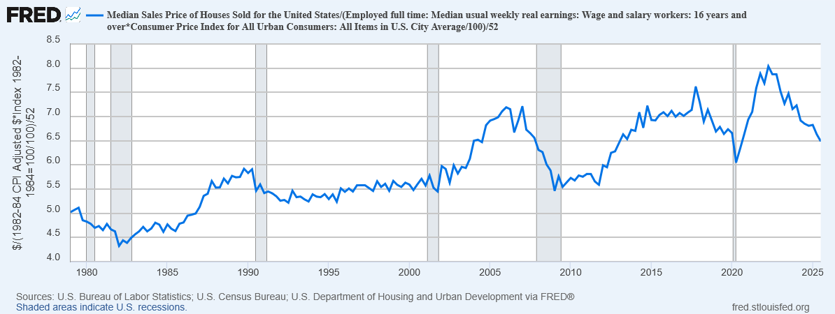
The graph below, constructed from FRED data, provides a simple measure of housing affordability: How many years of median earnings does it take to afford the median home?
From a low of 4.4 in 1982, this rose to about 5.5 and was relatively stable in the 1990s. Then in the 2000s, it began to rise, peaked at 7.2 just before the housing crisis, and then rapidly dropped to back to 5.5 again.
Then in the 2010s it began to rise again, peaked even higher at 7.6 in 2017, and then dropped down to 6.0 in 2020 before beginning to rise anew. In 2023 it reached a yet higher peak of 8.0, and then has been slowly declining ever since—but is still about 6.5, well above its 1990s level.
I honestly expected worse than this, but I think part of what’s happening is that new homes have gotten a bit smaller in the past few years: median square footage of homes sold has fallen from a peak of 1997 in 2019 to 1788 today. (Unfortunately, FRED doesn’t have this data series going back any earlier than 2016.)
If we adjust for that, the price a typical 2019 home today would be about 7.2 years of median earnings, which is about what it was at the peak of the housing crisis in 2007.
Note of course this isn’t actually how many years you need to save up to buy a house. You clearly can’t save your entire earnings, but you also don’t need to come up with the full price, only the down payment. And what you can afford also depends upon interest rates and such. But still, it’s a pretty clear sign that housing is radically more expensive now than it was in the 1980s or even 1990s.
In my view, this is the affordability crisis.
Gas prices really aren’t that important. Car prices are relatively stable. Food prices are volatile but don’t have a bad long-term trend. We do still have serious problems with affordability in education and healthcare, but we have obvious solutions available (that several other countries are already doing successfully); we’re just not doing them because Republicans don’t like them. But housing? We have no clear solutions on the table, certainly not anything that would be politically viable. Fundamentally, we need to build more housing in places people want to live—a lot more housing—and force the price of housing down.
And with our society structured the way it is, when you price people out of housing, you price them out of adulthood. Millennials are not having kids at anywhere near the rate of previous generations, because raising kids requires living space. Especially with immigration collapsing after Trump, this housing affordability crisis is going to turn into a population crisis.
I guess what I’m hoping for at the moment is just consciousness-raising, making people see that this is actually a problem. For some reason, everyone agrees that rising prices of goods are a bad thing, except when it comes to housing.
Inflation in food? An urgent crisis that must be immediately resolved.
Inflation in gas prices? So terrible it’s worth invading other countries over.
Inflation in housing? No, somehow that’s good actually, because it makes homeowners feel richer (even though they actually owe more in property taxes). We treat housing like an asset instead of a good, which is something we should absolutely never, ever do with a good that people need to live.
In last week’s post I described Philip E. Tetlock’s experiment showing that “foxes” (people who are open-minded and willing to consider alternative views) make more accurate predictions than “hedgehogs” (people who are dogmatic and conform strictly to a single ideology).
As I explained at the end of the post, he, uh, hedges on this point quite a bit, coming up with various ways that the hedgehogs might be able to redeem themselves, but still concluding that in most circumstances, the foxes seem to be more accurate.
Here are my thoughts on this:
I think he went too easy on the hedgehogs.
I consider myself very much a fox, and I honestly would never assign a probability of 0% or 100% to any physically possible event. Honestly I consider it a flaw in Tetlock’s design that he included those as options but didn’t include probabilities I would assign, like 1%, 0.1%, or 0.01%.
He only let people assign probabilities in 10% increments. So I guess if you thought something was 3% likely, you’re supposed to round to 0%? That still feels terrible. I’d probably still write 10%. There weren’t any questions like “Aliens from the Andromeda Galaxy arrive to conquer our planet, thus rendering all previous political conflicts moot”, but man, had there been, I’d still be tempted to not put 0%. I guess I would put 0% for that though? Because in 99.999999% of cases, I’d get it right—it wouldn’t happen—and I’d get more points. But man, even single-digit percentages? I’d mash the 10% button. I am pretty much allergic to overconfidence.
In fact, I think in my mind I basically try to use a logarithmic score, which unlike a Brier score, severely (technically, infinitely) punishes you for saying that something impossible happened or something inevitable didn’t. Like, really, if you’re doing it right, that should never, ever happen to you. If you assert that something has 0% probability and it happens, you have just conclusively disproven your worldview. (Admittedly it’s possible you could fix it with small changes—but a full discussion of that would get us philosophically too far afield. “outside the scope of this paper”.)
So honestly I think he was too lenient on overconfidence by using a Brier score, which does penalize this kind of catastrophic overconfidence, but only by a moderate amount. If you say that something has a 0% chance and then it happens, you get a Brier score of -1. But if you say that something has a 50% chance and then it happens (which it would, you know, 50% of the time), you’d get a Brier score of -0.25. So even absurd overconfidence isn’t really penalized that badly.
Compare this to a logarithmic rule: Say 0% and it happens, and you get negative infinity. You lose. You fail. Go home. Your worldview is bad and you should feel bad. This should never happen to you if you have a coherent worldview (modulo the fact that he didn’t let you say 0.01%).
So if I had designed this experiment, I would have given finer-grained options at the extremes, and then brought the hammer down on anybody who actually asserted a 0% chance of an event that actually occurred. (There’s no need for the finer-grained options elsewhere; over millennia of history, the difference between 0% and 0.1% is whether it won’t happen or it will—quite relevant for, say, full-scale nuclear war—while the difference between 40% and 42.1% is whether it’ll happen every 2 to 3 years or… every 2 to 3 years.)
But okay, let’s say we stick with the Brier score, because infinity is scary.
About the adjustments:
The “value adjustments” are just absolute nonsense. Those would be reasons to adjust your policy response, via your utility function—they are not a reason to adjust your probability. Yes, a nuclear terrorist attack would be a really big deal if it happened and we should definitely be taking steps to prevent that; but that doesn’t change the fact that the probability of one happening is something like 0.1% per year and none have ever happened. Predicting things that don’t happen is bad forecasting, even if the things you are predicting would be very important if they happened.
The “difficulty adjustments” are sort of like applying a different scoring rule, so that I’m more okay with; but that wasn’t enough to make the hedgehogs look better than the foxes.
The “fuzzy set” adjustments could be legitimate, but only under particular circumstances. Being “almost right” is only valid if you clearly showed that the result was anomalous because of some other unlikely event, and—because the timeframe was clearly specified in the questions—“might still happen” should still get fewer points than accurately predicting that it hasn’t happened yet. Moreover, it was very clear that people only ever applied these sort of changes when they got things wrong; they rarely if ever said things like “Oh, wow, I said that would happen and it did, but for completely different reasons that I didn’t expect—I was almost wrong there.” (Crazy example, but if the Soviet Union had been taken over by aliens, “the Soviet Union will fall” would be correct—but I don’t think you could really attribute that to good political prediction.)
The second exercise shows that even the foxes are not great Bayesians, and that some manipulations can make people even more inaccurate than before; but the hedgehogs also perform worse and also make some of the same crazy mistakes and still perform worse overall than the foxes, even in that experiment.
I guess he’d call me a “hardline neopositivist”? Because I think that your experiment asking people to predict things should require people to, um, actually predict things? The task was not to get the predictions wrong but be able to come up with clever excuses for why they were wrong that don’t challenge their worldview. The task was to not get the predictions wrong. Apparently this very basic level of scientific objectivity is now considered “hardline neopositivism”.
I guess we can reasonably acknowledge that making policy is about more than just prediction, and indeed maybe being consistent and decisive is advantageous in a game-theoretic sense (in much the same way that the way to win a game of Chicken is to very visibly throw away your steering wheel). So you could still make a case for why hedgehogs are good decision-makers or good leaders.
But I really don’t see how you weasel out of the fact that hedgehogs are really bad predictors. If I were running a corporation, or a government department, or an intelligence agency, I would want accurate predictions. I would not be interested in clever excuses or rich narratives. Maybe as leaders one must assemble such narratives in order to motivate people; so be it, there’s a division of labor there. Maybe I’d have a separate team of narrative-constructing hedgehogs to help me with PR or something. But the people who are actually analyzing the data should be people who are good at making accurate predictions, full stop.
And in fact, I don’t think hedgehogs are good decision-makers or good leaders. I think they are good politicians. I think they are good at getting people to follow them and believe what they say. But I do not think they are actually good at making the decisions that would be the best for society.
Indeed, I think this is a very serious problem.
I think we systematically elect people to higher office—and hire them for jobs, and approve them for tenure, and so on—because they express confidence rather than competence. We pick the people who believe in themselves the most, who (by regression to the mean if nothing else) are almost certainly the people who are most over-confident in themselves.
Given that confidence is easier to measure than competence in most areas, it might still make sense to choose confident people if confidence were really positively correlated with competence, but I’m not convinced that it is. I think part of what Tetlock is showing us is that the kind of cognitive style that yields high confidence—a hedgehog—simply is not the kind of cognitive style that yields accurate beliefs—a fox. People who are really good at their jobs are constantly questioning themselves, always open to new ideas and new evidence; but that also means that they hedge their bets, say “on the other hand” a lot, and often suffer from Impostor Syndrome. (Honestly, testing someone for Impostor Syndrome might be a better measure of competence than a traditional job interview! Then again, Goodhart’s Law.)
Indeed, I even see this effect within academic science; the best scientists I know are foxes through and through, but they’re never the ones getting published in top journals and invited to give keynote speeches at conferences. The “big names” are always hedgehog blowhards with some pet theory they developed in the 1980s that has failed to replicate but somehow still won’t die.
Moreover, I would guess that trustworthiness is actually pretty strongly inversely correlated to confidence—“con artist” is short for “confidence artist”, after all.
Then again, I tried to find rigorous research comparing openness (roughly speaking “fox-ness”) or humility to honesty, and it was surprisingly hard to find. Actually maybe the latter is just considered an obvious consensus in the literature, because there is a widely-used construct called honesty-humility. (In which case, yeah, my thinking on trustworthiness and confidence is an accepted fact among professional psychologists—but then, why don’t more people know that?)
But that still doesn’t tell me if there is any correlation between honesty-humility and openness.
Here’s a factor analysis specifically arguing for designing measures of honesty-humility so that they don’t correlate with other personality traits, so it can be seen as its own independent personality trait. There are some uncomfortable degrees of freedom in designing new personality metrics, which may make this sort of thing possible; and then by construction honesty-humility and openness would be uncorrelated, because any shared components were parceled out to one trait or the other.
So, I guess I can’t really confirm my suspicion here; maybe people who think like hedgehogs aren’t any less honest, or are even more honest, than people who think like foxes. But I’d still bet otherwise. My own life experience has been that foxes are honest and humble while hedgehogs are deceitful and arrogant.
Indeed, I believe that in systematically choosing confident hedgehogs as leaders, the world economy loses tens of trillions of dollars a year in inefficiencies. In fact, I think that we could probably end world hunger if we only ever put leaders in charge who were both competent and trustworthy.
Of course, in some sense that’s a pipe dream; we’re never going to get all good leaders, just as we’ll never get zero death or zero crime.
But based on how otherwise-similar countries have taken wildly different trajectories based on differences in leadership, I suspect that even relatively small changes in that direction could have quite large impacts on a society’s outcomes: South Korea isn’t perfect at picking its leaders; but surely it’s better than North Korea, and indeed that seems like one of the primary things that differentiates the two countries. Botswana is not a utopian paradise, but it’s a much nicer place to live than Nigeria, and a lot of the difference seems to come down to who is in charge, or who has been in charge for the last few decades.
And I could put in a jab here about the current state of the United States, but I’ll resist. If you read my blog, you already know my opinions on this matter.
Today I finally got around to reading Expert Political Judgment by Philip E. Tetlock, more or less in a single sitting because I’ve been sick the last week with some pretty tight limits on what activities I can do. (It’s mostly been reading, watching TV, or playing video games that don’t require intense focus.)
It’s really an excellent book, and I now both understand why it came so highly recommended to me, and now pass on that recommendation to you: Read it.
The central thesis of the book really boils down to three propositions:
Human beings, even experts, are very bad at predicting political outcomes.
Some people, who use an open-minded strategy (called “foxes”), perform substantially better than other people, who use a more dogmatic strategy (called “hedgehogs”).
When rewarding predictors with money, power, fame, prestige, and status, human beings systematically favor (over)confident “hedgehogs” over (correctly) humble “foxes”.
I decided I didn’t want to make this post about current events, but I think you’ll probably agree with me when I say:
That explains a lot.
How did Tetlock determine this?
Well, he studies the issue several different ways, but the core experiment that drives his account is actually a rather simple one:
He gathered a large group of subject-matter experts: Economists, political scientists, historians, and area-studies professors.
He came up with a large set of questions about politics, economics, and similar topics, which could all be formulated as a set of probabilities: “How likely is this to get better/get worse/stay the same?” (For example, this was in the 1980s, so he asked about the fate of the Soviet Union: “By 1990, will they become democratic, remain as they are, or collapse and fragment?”)
Each respondent answered a subset of the questions, some about their own particular field, some about another, more distant field; they assigned probabilities on an 11-point scale, from 0% to 100% in increments of 10%.
A few years later, he compared the predictions to the actual results, scoring them using a Brier score, which penalizes you for assigning high probability to things that didn’t happen or low probability to things that did happen.
He compared the resulting scores between people with different backgrounds, on different topics, with different thinking styles, and a variety of other variables. He also benchmarked them using some automated algorithms like “always say 33%” and “always give ‘stay the same’ 100%”.
I’ll show you the key results of that analysis momentarily, but to help it make more sense to you, let me elaborate a bit more on the “foxes” and “hedgehogs”. The notion is was first popularized by Isaiah Berlin in an essay called, simply, The Hedgehog and the Fox.
“The fox knows many things, but the hedgehog knows one very big thing.”
That is, someone who reasons as a “fox” combines ideas from many different sources and perspective, and tries to weigh them all together into some sort of synthesis that then yields a final answer. This process is messy and complicated, and rarely yields high confidence about anything.
Whereas, someone who reasons as a “hedgehog” has a comprehensive theory of the world, an ideology, that provides clear answers to almost any possible question, with the surely minor, insubstantial flaw that those answers are not particularly likely to be correct.
He also considered “hedge-foxes” (people who are mostly fox but also a little bit hedgehog) and “fox-hogs” (people who are mostly hedgehog but also a little bit fox).
Tetlock has decomposed the scores into two components: calibration and discrimination. (Both very overloaded words, but they are standard in the literature.)
Calibration is how well your stated probabilities matched up with the actual probabilities; that is, if you predicted 10% probability on 20 different events, you have very good calibration if precisely 2 of those events occurred, and very poor calibration if 18 of those events occurred.
Discrimination more or less describes how useful your predictions are, what information they contain above and beyond the simple base rate. If you just assign equal probability to all events, you probably will have reasonably good calibration, but you’ll have zero discrimination; whereas if you somehow managed to assign 100% to everything that happened and 0% to everything that didn’t, your discrimination would be perfect (and we would have to find out how you cheated, or else declare you clairvoyant).
For both measures, higher is better. The ideal for each is 100%, but it’s virtually impossible to get 100% discrimination and actually not that hard to get 100% calibration if you just use the base rates for everything.
There is a bit of a tradeoff between these two: It’s not too hard to get reasonably good calibration if you just never go out on a limb, but then your predictions aren’t as useful; we could have mostly just guessed them from the base rates.
On the graph, you’ll see downward-sloping lines that are meant to represent this tradeoff: Two prediction methods that would yield the same overall score but different levels of calibration and discrimination will be on the same line. In a sense, two points on the same line are equally good methods that prioritize usefulness over accuracy differently.
All right, let’s see the graph at last:
The pattern is quite clear: The more foxy you are, the better you do, and the more hedgehoggy you are, the worse you do.
I’d also like to point out the other two regions here: “Mindless competition” and “Formal models”.
The former includes really simple algorithms like “always return 33%” or “always give ‘stay the same’ 100%”. These perform shockingly well. The most sophisticated of these, “case-specific extrapolation” (35 and 36 on the graph, which basically assumes that each country will continue doing what it’s been doing) actually performs as well if not better than even the foxes.
And what’s that at the upper-right corner, absolutely dominating the graph? That’s “Formal models”. This describes basically taking all the variables you can find and shoving them into a gigantic logit model, and then outputting the result. It’s computationally intensive and requires a lot of data (hence why he didn’t feel like it deserved to be called “mindless”), but it’s really not very complicated, and it’s the best prediction method, in every way, by far.
This has made me feel quite vindicated about a weird nerd thing I do: When I have a big decision to make (especially a financial decision), I create a spreadsheet and assemble a linear utility model to determine which choice will maximize my utility, under different parameterizations based on my past experiences. Whichever result seems to win the most robustly, I choose. This is fundamentally similar to the “formal models” prediction method, where the thing I’m trying to predict is my own happiness. (It’s a bit less formal, actually, since I don’t have detailed happiness data to feed into the regression.) And it has worked for me, astonishingly well. It definitely beats going by my own gut. I highly recommend it.
What does this mean?
Well first of all, it means humans suck at predicting things.At least for this data set, even our experts don’t perform substantially better than mindless models like “always assume the base rate”.
Nor do experts perform much better in their own fields than in other fields; they do all perform better than undergrads or random people (who somehow perform worse than the “mindless” models)
But Tetlock also investigates further, trying to better understand this “fox/hedgehog” distinction and why it yields different performance. He really bends over backwards to try to redeem the hedgehogs, in the following ways:
He allows them to make post-hoc corrections to their scores, based on “value adjustments” (assigning higher probability to events that would be really important) and “difficulty adjustments” (assigning higher scores to questions where the three outcomes were close to equally probable) and “fuzzy sets” (giving some leeway on things that almost happened or things that might still happen later).
He demonstrates a different, related experiment, in which certain manipulations can cause foxes to perform a lot worse than they normally would, and even yield really crazy results like probabilities that add up to 200%.
He has a whole chapter that is a Socratic dialogue (seriously!) between four voices: A “hardline neopositivist”, a “moderate neopositivist”, a “reasonable relativist”, and an “unrelenting relativist”; and all but the “hardline neopositivist” agree that there is some legitimate place for the sort of post hoc corrections that the hedgehogs make to keep themselves from looking so bad.
This post is already getting a bit long, so that will conclude part I. Stay tuned for part II, next week!
In last week’s post I constructed an Index of National Expenditure (INE), attempting to estimate the total cost of all of the things a family needs and can’t do without, like housing, food, clothing, cars, healthcare, and education. What I found shocked me: The median family cannot afford all necessary expenditures.
I have a couple more thoughts about that.
I still don’t understand why people care so much about gas prices.
Gasoline was a relatively small contribution to INE. It was more than clothing but less than utilities, and absolutely dwarfed by housing, food, or college. I thought maybe since I only counted a 15-mile commute, maybe I didn’t actually include enoughgasoline usage, but based on this estimate of about $2000 per driver, I was in about the right range; my estimate for the same year was $3350 for a 2-car family.
I think I still have to go with my salience hypothesis: Gasoline is the only price that we plaster in real-time on signs on the side of the road. So people are constantly aware of it, even though it isn’t actually that important.
The price surge that should be upsetting people is housing.
If the price of homes had only risen with the rate of CPI inflation instead of what it actually did, the median home price in 2024 would be only $234,000 instead of the $396,000 it actually is; and by my estimation that would save a typical family $11,000 per year—a whopping 15% of their income, and nearly enough to make the INE affordable by itself.
Now, I’ll consider some possible objections to my findings.
Objection 1: A typical family doesn’t actually spend this much on these things.
You’re right, they don’t! Because they couldn’t possibly. Even with substantial debt, you just can’t sustainably spend 125% of your after-tax household income.
My goal here was not to estimate how much families actually spend; it was to estimate how much they need to spend in order to live a good life and not feel deprived.
What I have found is that most American families feel deprived. They are forced to sacrifice something really important—like healthcare, or education, or owning a home—because they simply can’t afford it.
What I’m trying to do here is find the price of the American Dream; and what I’ve found is that the American Dream has a price that most Americans cannot afford.
Objection 2: You should use median healthcare spending, not mean.
I did in fact use mean figures instead of median for healthcare expenditures, mainly because only the mean was readily available. Mean income is higher than median income, so you might say that I’ve overestimated healthcare expenditure—and in a sense that’s definitely true. The median family spends less than this on healthcare.
But the reason that the median family spends less than this on healthcare is not that they want to, but that they have to. Healthcare isn’t a luxury that people buy more of because they are richer. People buy either as much as they need or as much as they can afford—whichever is lower, which is typically the latter. Using the mean instead of the median is a crude way to account for that, but I think it’s a defensible one.
But okay, let’s go ahead and cut the estimate of healthcare spending in half; even if you do that, the INE is still larger than after-tax median household income in most years.
Objection 3: A typical family isn’t a family of four, it’s a family of three.
Part of what I seem to be finding here is that a family of four is unaffordable—literally impossible to afford—on a typical family income.
But a healthy society is one in which typical families have two or three children. That is what we need in order to achieve population replacement. When families get smaller than that, we aren’t having enough children, and our population will decline—which means that we’ll have too many old people relative to young people. This puts enormous pressure on healthcare and pension systems, which rely upon the fact that young people produce more, in order to pay for the fact that old people cost more.
This is bad. This is not sustainable. If the reason families aren’t having enough kids is that they can’t afford them—and this fits with other research on the subject—then this economic failure damages our entire society, and it needs to be fixed.
Objection 4: Many families buy their cars used.
Perhaps 1/10 of a new car every year isn’t an ideal estimate of how much people spend on their cars, but if anything I think it’s conservative, because if you only buy a car every 10 years, and it was already used when you bought it, you’re going to need to spend a lot on maintaining it—quite possibly more than it would cost to get a new one. Motley Fool actually estimates the ownership cost of just one car at substantially more than I estimated for two cars. So if anything your complaint should be that I’ve underestimated the cost by not adequately including maintenance and insurance.
Objection 5: Not everyone gets a four-year college degree.
Fair enough; a substantial proportion get associate’s degrees, and most people get no college degree at all. But some also get graduate degrees, which is even more expensive (ask me how I know).
Moreover, in today’s labor market, having a college degree makes a huge difference in your future earnings; a bachelor’s degree increases your lifetime earnings by a whopping 84%. In theory it’s okay to have a society where most people don’t go to college; in practice, in our society, not going to college puts you at a tremendous disadvantage for the rest of your life. So we either need to find a way to bring wages up for those who don’t go to college, or find a way to bring the cost of college down.
This is probably one of the things that families actually choose to scrimp on, only sending one kid to college or none at all. But because college is such a huge determinant of earnings, this perpetuates intergenerational inequality: Only rich families can afford to send their kids to college, and only kids who went to college grow up to have rich families.
Objection 6: You don’t actually need to save for college; you can use student loans.
Yes, you can, and in practice, most people who to college do. But while this solves the liquidity problem (having enough money right now), it does not solve the solvency problem (having enough money in the long run). Failing to save for college and relying on student loans just means pushing the cost of college onto your children—and since we’ve been doing that for over a generation, feel free to replace the category “college savings” with “repaying student loans”; it won’t meaningfully change the results.
I’m still reeling from the fact that Donald Trump was re-elected President. He seemed obviously horrible at the time, and he still seems horrible now, for many of the same reasons as before (we all knew the tariffs were coming, and I think deep down we knew he would sell out Ukraine because he loves Putin), as well as some brand new ones (I did not predict DOGE would gain access to all the government payment systems, nor that Trump would want to start a “crypto fund”). Kamala Harris was not an ideal candidate, but she was a good candidate, and the comparison between the two could not have been starker.
Now that the dust has cleared and we have good data on voting patterns, I am now less convinced than I was that racism and sexism were decisive against Harris. I think they probably hurt her some, but given that she actually lost the most ground among men of color, racism seems like it really couldn’t have been a big factor. Sexism seems more likely to be a significant factor, but the fact that Harris greatly underperformed Hillary Clinton among Latina women at least complicates that view.
A lot of voters insisted that they voted on “inflation” or “the economy”. Setting aside for a moment how absurd it was—even at the time—to think that Trump (he of the tariffs and mass deportations!) was going to do anything beneficial for the economy, I would like to better understand how people could be so insistent that the economy was bad even though standard statistical measures said it was doing fine.
Krugman believes it was a “vibecession”, where people thought the economy was bad even though it wasn’t. I think there may be some truth to this.
But today I’d like to evaluate another possibility, that what people were really reacting against was not inflation per se but necessitization.
I first wrote about necessitization in 2020; as far as I know, the term is my own coinage. The basic notion is that while prices overall may not have risen all that much, prices of necessities have risen much faster, and the result is that people feel squeezed by the economy even as CPI growth remains low.
In this post I’d like to more directly evaluate that notion, by constructing an index of necessary expenditure (INE).
The core idea here is this:
What would you continue to buy, in roughly the same amounts, even if it doubled in price, because you simply can’t do without it?
For example, this is clearly true of housing: You can rent or you can own, but can’t not have a house. And nor are most families going to buy multiple houses—and they can’t buy partial houses.
It’s also true of healthcare: You need whatever healthcare you need. Yes, depending on your conditions, you maybe could go without, but not without suffering, potentially greatly. Nor are you going to go out and buy a bunch of extra healthcare just because it’s cheap. You need what you need.
I think it’s largely true of education as well: You want your kids to go to college. If college gets more expensive, you might—of necessity—send them to a worse school or not allow them to complete their degree, but this would feel like a great hardship for your family. And in today’s economy you can’t not send your kids to college.
But this is not true of technology: While there is a case to be made that in today’s society you need a laptop in the house, the fact is that people didn’t used to have those not that long ago, and if they suddenly got a lot cheaper you very well might buy another one.
Well, it just so happens that housing, healthcare, and education have all gotten radically more expensive over time, while technology has gotten radically cheaper. So prima facie, this is looking pretty plausible.
But I wanted to get more precise about it. So here is the index I have constructed. I consider a family of four, two adults, two kids, making the median household income.
To get the median income, I’ll use this FRED series for median household income, then use this table of median federal tax burden to get an after-tax wage. (State taxes vary too much for me to usefully include them.) Since the tax table ends in 2020 which was anomalous, I’m going to extrapolate that 2021-2024 should be about the same as 2019.
I assume the kids go to public school, but the parents are saving up for college; to make the math simple, I’ll assume the family is saving enough for each kid to graduate from with a four-year degree from a public university, and that saving is spread over 16 years of the child’s life. 2*4/16 = 0.5; this means that each year the family needs to come up with 0.5 years of cost of attendance. (I had to get the last few years from here, but the numbers are comparable.)
I assume the family owns two cars—both working full time, they kinda have to—which I amortize over 10 year lifetimes; 2*1/10 = 0.2, so each year the family pays 0.2 times the value of an average midsize car. (The current average new car price is $33226; I then use the CPI for cars to figure out what it was in previous years.)
I assume they pay a 30-year mortgage on the median home; they would pay interest on this mortgage, so I need to factor that in. I’ll assume they pay the average mortgage rate in that year, but I don’t want to have to do a full mortgage calculation (including PMI, points, down payment etc.) for each year, so I’ll say that they amount they pay is (1/30 + 0.5 (interest rate))*(home value) per year, which seems to be a reasonable approximation over the relevant range.
I assume that both adults have a 15-mile commute (this seems roughly commensurate with the current mean commute time of 26 minutes), both adults work 5 days per week, 50 weeks per year, and their cars get the median level of gas mileage. This means that they consume 2*15*2*5*50/(median MPG) = 15000/(median MPG) gallons of gasoline per year. I’ll use this BTS data for gas mileage. I’m intentionally not using median gasoline consumption, because when gas is cheap, people might take more road trips, which is consumption that could be avoided without great hardship when gas gets expensive. I will also assume that the kids take the bus to school, so that doesn’t contribute to the gasoline cost.
That I will multiply by the average price of gasoline in June of that year, which I have from the EIA since 1993. (I’ll extrapolate 1990-1992 as the same as 1993, which is conservative.)
I will assume that the family owns 2 cell phones, 1 computer, and 1 television. This is tricky, because the quality of these tech items has dramatically increased over time.
If you try to measure with equivalent buying power (e.g. a 1 MHz computer, a 20-inch CRT TV), then you’ll find that these items have gotten radically cheaper; $1000 in 1950 would only buy as much TV as $7 today, and a $50 Raspberry Pi‘s 2.4 GHz processor is 150 times faster than the 16 MHz offered by an Apple Powerbook in 1991—despite the latter selling for $2500 nominally. So in dollars per gigahertz, the price of computers has fallen by an astonishing 7,500 times just since 1990.
But I think that’s an unrealistic comparison. The standards for what was considered necessary have also increased over time. I actually think it’s quite fair to assume that people have spent a roughly constant nominal amount on these items: about $500 for a TV, $1000 for a computer, and $500 for a cell phone. I’ll also assume that the TV and phones are good for 5 years while the computer is good for 2 years, which makes the total annual expenditure for 2 phones, a TV, and a computer equal to 2/5*500 + 1/5*500 + 1/2*1000 = 800. This is about what a family must spend every year to feel like they have an adequate amount of digital technology.
I will assume that the family buys the equivalent of five months of infant care per year; they surely spend more than this (in either time or money) when they have actual infants, but less as the kids grow. This amounts to about $5000 today, but was only $1600 in 1990—a 214% increase, or 3.42% per year.
For food expenditure, I’m going to use the USDA’s thrifty plan for June of that year. I’ll use the figures assuming that one child is 6 and the other is 9. I don’t have data before 1994, so I’ll extrapolate that with the average growth rate of 3.2%.
The figures I had the hardest time getting were for utilities. It’s also difficult to know what to include: Is Internet access a necessity? Probably, nowadays—but not in 1990. Should I separate electric and natural gas, even though they are partial substitutes? But using these figures I estimate that utility costs rise at about 0.8% per year in CPI-adjusted terms, so what I’ll do is benchmark to $3800 in 2016 and assume that utility costs have risen by (0.8% + inflation rate) per year each year.
Healthcare is also a tough one; pardon the heteronormativity, but for simplicity I’m going to use the mean personal healthcare expenditures for one man and woman (aged 19-44) and one boy and one girl (aged 0-18). Unfortunately I was only able to find that for two-year intervals in the range from 2002 to 2020, so I interpolated and extrapolated both directions assuming the same average growth rate of 3.5%.
So let’s summarize what all is included here:
Estimated payment on a mortgage
0.5 years of college tuition
amortized cost of 2 cars
7500/(median MPG) gallons of gasoline
amortized cost of 2 phones, 1 computer, and 1 television
average spending on clothes
11% of income on food
Estimated utilities spending
Estimated childcare equivalent to five months of infant care
Healthcare for one man, one woman, one boy, one girl
There are obviously many criticisms you could make of these choices. If I were writing a proper paper, I would search harder for better data and run robustness checks over the various estimation and extrapolation assumptions. But for these purposes I really just want a ballpark figure, something that will give me a sense of what rising cost of living feels like to most people.
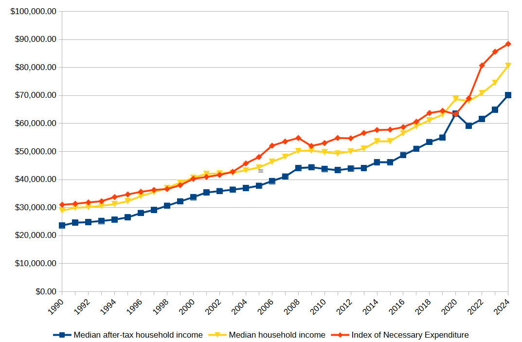
What I found absolutely floored me. Over the range from 1990 to 2024:
The Index of Necessary Expenditure rose by an average of 3.45% per year, almost a full percentage point higher than the average CPI inflation of 2.62% per year.
Over the same period, after-tax income rose at a rate of 3.31%, faster than CPI inflation, but slightly slower than the growth rate of INE.
The Index of Necessary Expenditure was over 100% of median after-tax household income every year except 2020.
Since 2021, the Index of Necessary Expenditure has risen at an average rate of 5.74%, compared to CPI inflation of only 2.66%. In that same time, after-tax income has only grown at a rate of 4.94%.
Point 3 is the one that really stunned me. The only time in the last 34 years that a family of four has been able to actually pay for all necessities—just necessities—on a typical household income was during the COVID pandemic, and that in turn was only because the federal tax burden had been radically reduced in response to the crisis. This means that every single year, a typical American family has been either going further and further into debt, or scrimping on something really important—like healthcare or education.
No wonder people feel like the economy is failing them! It is!
In fact, I can even make sense now of how Trump could convince people with “Are you better off than you were four years ago?” in 2024 looking back at 2020—while the pandemic was horrific and the disruption to the economy was massive, thanks to the US government finally actually being generous to its citizens for once, people could just about actually make ends meet. That one year. In my entire life.
This is why people felt betrayed by Biden’s economy. For the first time most of us could remember, we actually had this brief moment when we could pay for everything we needed and still have money left over. And then, when things went back to “normal”, it was taken away from us. We were back to no longer making ends meet.
When I went into this, I expected to see that the INE had risen faster than both inflation and income, which was indeed the case. But I expected to find that INE was a large but manageable proportion of household income—maybe 70% or 80%—and slowly growing. Instead, I found that INE was greater than 100% of income in every year but one.
And the truth is, I’m not sure I’ve adequately covered all necessary spending! My figures for childcare and utilities are the most uncertain; those could easily go up or down by quite a bit. But even if I exclude them completely, the reduced INE is still greater than income in most years.
Suddenly the way people feel about the economy makes a lot more sense to me.
I don’t think most Americans realize just how much more the US spends on healthcare than other countries. This is true not simply in absolute terms—of course it is, the US is rich and huge—but in relative terms: As a portion of GDP, our healthcare spending is a major outlier.
Here’s a really nice graph from Healthsystemtracker.org that illustrates it quite nicely: Almost all other First World countries share a simple linear relationship between their per-capita GDP and their per-capita healthcare spending. But one of these things is not like the other ones….
The outlier in the other direction is Ireland, but that’s because their GDP is wildly inflated by Leprechaun Economics. (Notice that it looks like Ireland is by far the richest country in the sample! This is clearly not the case in reality.) With a corrected estimate of their true economic output, they are also quite close to the line.
Since US GDP per capita ($70,181) is in between that of Denmark ($64,898) and Norway ($80,496) both of which have very good healthcare systems (#ScandinaviaIsBetter), we would expect that US spending on healthcare would similarly be in between. But while Denmark spends $6,384 per person per year on healthcare and Norway spends $7,065 per person per year, the US spends $12,914.
That is, the US spends nearly twice as much as it should on healthcare.
The absolute difference between what we should spend and what we actually spend is nearly $6,000 per person per year. Multiply that out by the 330 million people in the US, and…
The US overspends on healthcare by nearly $2 trillion per year.
This might be worth it, if health in the US were dramatically better than health in other countries. (In that case I’d be saying that other countries spend too little.) But plainly it is not.
Probably the simplest and most comparable measure of health across countries is life expectancy. US life expectancy is 76 years, and has increased over time. But if you look at the list of countries by life expectancy, the US is not even in the top 50. Our life expectancy looks more like middle-income countries such as Algeria, Brazil, and China than it does like Norway or Sweden, who should be our economic peers.
There are of course many things that factor into life expectancy aside from healthcare: poverty and homicide are both much worse in the US than in Scandinavia. But then again, poverty is much worse in Algeria, and homicide is much worse in Brazil, and yet they somehow manage to nearly match the US in life expectancy (actually exceeding it in some recent years).
The US somehow manages to spend more on healthcare than everyone else, while getting outcomes that are worse than any country of comparable wealth—and even some that are far poorer.
This is largely why there is a so-called “entitlements crisis” (as many a libertarian think tank is fond of calling it). Since libertarians want to cut Social Security most of all, they like to lump it in with Medicare and Medicaid as an “entitlement” in “crisis”; but in fact we only need a few minor adjustments to the tax code to make sure that Social Security remains solvent for decades to come. It’s healthcare spending that’s out of control.
Here, take a look.
This is the ratio of Social Security spending to GDP from 1966 to the present. Notice how it has been mostly flat since the 1980s, other than a slight increase in the Great Recession.
This is the ratio of Medicare spending to GDP over the same period. Even ignoring the first few years while it was ramping up, it rose from about 0.6% in the 1970s to almost 4% in 2020, and only started to decline in the last few years (and it’s probably too early to say whether that will continue).
Medicaid has a similar pattern: It rose steadily from 0.2% in 1966 to over 3% today—and actually doesn’t even show any signs of leveling off.
If you look at Medicare and Medicaid together, they surged from just over 1% of GDP in 1970 to nearly 7% today:
Put another way: in 1982, Social Security was 4.8% of GDP while Medicare and Medicaid combined were 2.4% of GDP. Today, Social Security is 4.9% of GDP while Medicare and Medicaid are 6.8% of GDP.
Social Security spending barely changed at all; healthcare spending more than doubled. If we reduced our Medicare and Medicaid spending as a portion of GDP back to what it was in 1982, we would save 4.4% of GDP—that is, 4.4% of over $25 trillion per year, so $1.1 trillion per year.
Of course, we can’t simply do that; if we cut benefits that much, millions of people would suddenly lose access to healthcare they need.
The problem is not that we are spending frivolously, wasting the money on treatments no one needs. On the contrary, both Medicare and Medicaid carefully vet what medical services they are willing to cover, and if anything probably deny services more often than they should.
No, the problem runs deeper than this.
Healthcare is too expensive in the United States.
We simply pay more for just about everything, and especially for specialist doctors and hospitals.
In most other countries, doctors are paid like any other white-collar profession. They are well off, comfortable, certainly, but few of them are truly rich. But in the US, we think of doctors as an upper-class profession, and expect them to be rich.
Median doctor salaries are $98,000 in France and $138,000 in the UK—but a whopping $316,000 in the US. Germany and Canada are somewhere in between, at $183,000 and $195,000 respectively.
Nurses, on the other hand, are paid only a little more in the US than in Western Europe. This means that the pay difference between doctors and nurses is much higher in the US than most other countries.
US prices on brand-name medication are frankly absurd. Our generic medications are typically cheaper than other countries, but our brand name pills often cost twice as much. I noticed this immediately on moving to the UK: I had always been getting generics before, because the brand name pills cost ten times as much, but when I moved here, suddenly I started getting all brand-name medications (at no cost to me), because the NHS was willing to buy the actual brand name products, and didn’t have to pay through the nose to do so.
Let’s compare the prices of a few inpatient procedures between the US and Switzerland. Switzerland, you should note, is a very rich country that spends a lot on healthcare and has nearly the world’s highest life expectancy. So it’s not like they are skimping on care. (Nor is it that prices in general are lower in Switzerland; on the contrary, they are generally higher.)
A coronary bypass in Switzerland costs about $33,000. In the US, it costs $76,000.
A spinal fusion in Switzerland costs about $21,000. In the US? $52,000.
Angioplasty in Switzerland: $9.000. In the US? $32,000.
Hip replacement: Switzerland? $16,000. The US? $28,000.
Knee replacement: Switzerland? $19,000. The US? $27,000.
Cholecystectomy: Switzerland? $8,000. The US? $16,000.
Appendectomy: Switzerland? $7,000. The US? $13,000.
Caesarian section: Switzerland? $8,000. The US? $11,000.
Hospital prices are even lower in Germany and Spain, whose life expectancies are not as high as Switzerland—but still higher than the US.
These prices are so much lower that in fact if you were considering getting surgery for a chronic condition in the US, don’t. Buy plane tickets to Europe and get the procedure done there. Spend an extra few thousand dollars on a nice European vacation and you’d still end up saving money. (Obviously if you need it urgently you have no choice but to use your nearest hospital.) I know that if I ever need a knee replacement (which, frankly, is likely, given my height), I’m gonna go to Spain and thereby save $22,000 relative to what it would cost in the US. That’s a difference of a car.
Combine this with the fact that the US is the only First World country without universal healthcare, and maybe you can see why we’re also the only country in the world where people are afraid to call an ambulance because they don’t think they can afford it. We are also the only country in the world with a medical debt crisis.
Where is all this extra money going?
Well, a lot of it goes to those doctors who are paid three times as much as in France. That, at least, seems defensible: If we want the best doctors in the world maybe we need to pay for them. (Then again, do we have the best doctors in the world? If so, why is our life expectancy so mediocre?)
But a significant portion is going to shareholders.
I was surprised to find that the US is not unusual in that; in fact, for-profit hospitals exist in dozens of countries, and the fraction of US hospital capacity that is for-profit isn’t even particularly high by world standards.
Even nonprofit US hospitals are tremendously profitable—as oxymoronic as that may sound. In fact, mean operating profit is higher among nonprofit hospitals in the US than for-profit hospitals. So even the hospitals that aren’t supposed to be run for profit… pretty much still are. They get tax deductions as if they were charities—but they really don’t act like charities.
They are basically nonprofitin name only.
So fixing this will not be as simple as making all hospitals nonprofit. We must also restructure the institutions so that nonprofit hospitals are genuinely nonprofit, and no longer nonprofit in name only. It’s normal for a nonprofit to have a little bit of profit or loss—nobody can make everything always balance perfectly—but these hospitals have been raking in huge profits and keeping it all in cash instead of using it to reduce prices or improve services. In the study I linked above, those 2,219 “nonprofit” hospitals took in operating profits averaging $43 million each—for a total of $95 billion.
Between pharmaceutical companies and hospitals, that’s a total of over $170 billion per year just in profit. (That’s more than we spend on food stamps, even after surge due to COVID.) This is pure grift. It must be stopped.
But that still doesn’t explain why we’re spending $2 trillion more than we should! So after all, I must leave you with a question:
What is America doing wrong? Why is our healthcare so expensive?
I wasn’t able to find a dictionary that includes the word “statisticacy”, but it doesn’t trigger my spell-check, and it does seem to have the same form as “numeracy”: numeric, numerical, numeracy, numerate; statistic, statistical, statisticacy, statisticate. It definitely still sounds very odd to my ears. Perhaps repetition will eventually make it familiar.
For the concept is clearly a very important one. Literacy and numeracy are no longer a serious problem in the First World; basically every adult at this point knows how to read and do addition. Even worldwide, 90% of men and 83% of women can read, at least at a basic level—which is an astonishing feat of our civilization by the way, well worthy of celebration.
But I have noticed a disturbing lack of, well, statisticacy. Even intelligent, educated people seem… pretty bad at understanding statistics.
I’m not talking about sophisticated econometrics here; of course most people don’t know that, and don’t need to. (Most economists don’t know that!) I mean quite basic statistical knowledge.
As part of being a good citizen in a modern society, every adult should understand the following:
1. The difference between a mean and a median, and why average income (mean) can increase even though most people are no richer (median).
2. The difference between increasing by X% and increasing by X percentage points: If inflation goes from 4% to 5%, that is an increase of 20% ((5/4-1)*100%), but only 1 percentage point (5%-4%).
3. The meaning of standard error, and how to interpret error bars on a graph—and why it’s a huge red flag if there aren’t any error bars on a graph.
4. Basic probabilistic reasoning: Given some scratch paper, a pen, and a calculator, everyone should be able to work out the odds of drawing a given blackjack hand, or rolling a particular number on a pair of dice. (If that’s too easy, make it a poker hand and four dice. But mostly that’s just more calculation effort, not fundamentally different.)
5. The meaning of exponential growth rates, and how they apply to economic growth and compound interest. (The difference between 3% interest and 6% interest over 30 years is more than double the total amount paid.)
I see people making errors about this sort of thing all the time.
Economic news that celebrates rising GDP but wonders why people aren’t happier (when real median income has been falling since 2019 and is only 7% higher than it was in 1999, an annual growth rate of 0.2%).
Reports on inflation, interest rates, or poll numbers that don’t clearly specify whether they are dealing with percentages or percentage points. (XKCD made fun of this.)
Speaking of poll numbers, any reporting on changes in polls that isn’t at least twice the margin of error of the polls in question. (There’s also a comic for this; this time it’s PhD Comics.)
And, perhaps worst of all, the plague of science news articles about “New study says X”. Things causing and/or cancer, things correlated with personality types, tiny psychological nudges that supposedly have profound effects on behavior.
Some of these things will even turn out to be true; actually I think this one on fibromyalgia, this one on smoking, and this one on body image are probably accurate. But even if it’s a properly randomized experiment—and especially if it’s just a regression analysis—a single study ultimately tells us very little, and it’s irresponsible to report on them instead of telling people the extensive body of established scientific knowledge that most people still aren’t aware of.
Basically any time an article is published saying “New study says X”, a statisticate person should ignore it and treat it as random noise. This is especially true if the finding seems weird or shocking; such findings are far more likely to be random flukes than genuine discoveries. Yes, they could be true, but one study just doesn’t move the needle that much.
I don’t remember where it came from, but there is a saying about this: “What is in the textbooks is 90% true. What is in the published literature is 50% true. What is in the press releases is 90% false.” These figures are approximately correct.
If their goal is to advance public knowledge of science, science journalists would accomplish a lot more if they just opened to a random page in a mainstream science textbook and started reading it on air. Admittedly, I can see how that would be less interesting to watch; but then, their job should be to find a way to make it interesting, not to take individual studies out of context and hype them up far beyond what they deserve. (Bill Nye did this much better than most science journalists.)
I’m not sure how much to blame people for lacking this knowledge. On the one hand, they could easily look it up on Wikipedia, and apparently choose not to. On the other hand, they probably don’t even realize how important it is, and were never properly taught it in school even though they should have been. Many of these things may even be unknown unknowns; people simply don’t realize how poorly they understand. Maybe the most useful thing we could do right now is simply point out to people that these things are important, and if they don’t understand them, they should get on that Wikipedia binge as soon as possible.
And one last thing: Maybe this is asking too much, but I think that a truly statisticate person should be able to solve the Monty Hall Problem and not be confused by the result. (Hint: It’s very important that Monty Hall knows which door the car is behind, and would never open that one. If he’s guessing at random and simply happens to pick a goat, the correct answer is 1/2, not 2/3. Then again, it’s never a bad choice to switch.)
Why are some molecules (e.g. DNA) billions of times larger than others (e.g. H2O), but all atoms are within a much narrower range of sizes (only a few hundred)?
Why are some animals (e.g. elephants) millions of times as heavy as other (e.g. mice), but their cells are basically the same size?
Why does capital income vary so much more (factors of thousands or millions) than wages (factors of tens or hundreds)?
These three questions turn out to have much the same answer: Scalability.
Atoms are not very scalable: Adding another proton to a nucleus causes interactions with all the other protons, which makes the whole atom unstable after a hundred protons or so. But molecules, particularly organic polymers such as DNA, are tremendously scalable: You can add another piece to one end without affecting anything else in the molecule, and keep on doing that more or less forever.
Cells are not very scalable: Even with the aid of active transport mechanisms and complex cellular machinery, a cell’s functionality is still very much limited by its surface area. But animals are tremendously scalable: The same exponential growth that got you from a zygote to a mouse only needs to continue a couple years longer and it’ll get you all the way to an elephant. (A baby elephant, anyway; an adult will require a dozen or so years—remarkably comparable to humans, in fact.)
Labor income is not very scalable: There are only so many hours in a day, and the more hours you work the less productive you’ll be in each additional hour. But capital income is perfectly scalable: We can add another digit to that brokerage account with nothing more than a few milliseconds of electronic pulses, and keep doing that basically forever (due to the way integer storage works, above 2^63 it would require special coding, but it can be done; and seeing as that’s over 9 quintillion, it’s not likely to be a problem any time soon—though I am vaguely tempted to write a short story about an interplanetary corporation that gets thrown into turmoil by an integer overflow error).
This isn’t just an effect of our accounting either. Capital is scalable in a way that labor is not. When your contribution to production is owning a factory, there’s really nothing to stop you from owning another factory, and then another, and another. But when your contribution is working at a factory, you can only work so hard for so many hours.
When a phenomenon is highly scalable, it can take on a wide range of outcomes—as we see in molecules, animals, and capital income. When it’s not, it will only take on a narrow range of outcomes—as we see in atoms, cells, and labor income.
Exponential growth is also part of the story here: Animals certainly grow exponentially, and so can capital when invested; even some polymers function that way (e.g. under polymerase chain reaction). But I think the scalability is actually more important: Growing rapidly isn’t so useful if you’re going to immediately be blocked by a scalability constraint. (This actually relates to the difference between r- and K- evolutionary strategies, and offers further insight into the differences between mice and elephants.) Conversely, even if you grow slowly, given enough time, you’ll reach whatever constraint you’re up against.
Indeed, we can even say something about the probability distribution we are likely to get from random processes that are scalable or non-scalable.
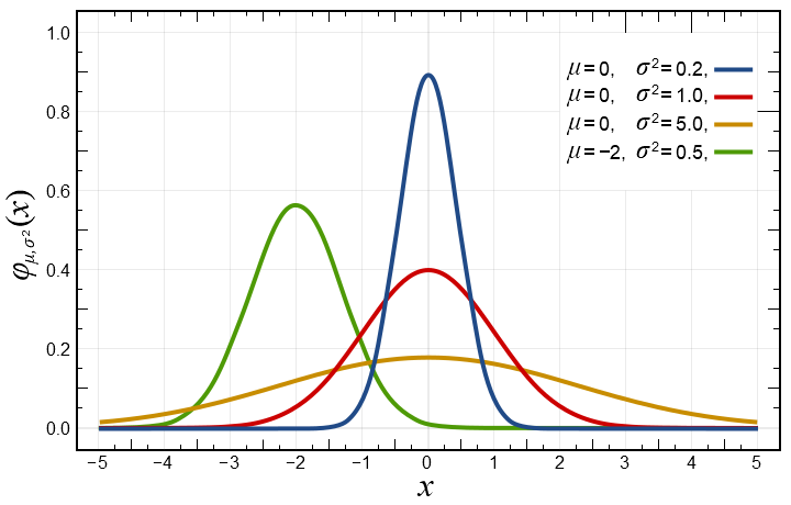
A non-scalable random process will generally converge toward the familiar normal distribution, a “bell curve”:
The normal distribution has most of its weight near the middle; most of the population ends up near there. This is clearly the case for labor income: Most people are middle class, while some are poor and a few are rich.
But a scalable random process will typically converge toward quite a different distribution, aPareto distribution:
A Pareto distribution has most of its weight near zero, but covers an extremely wide range. Indeed it is what we call fat tailed, meaning that really extreme events occur often enough to have a meaningful effect on the average. A Pareto distribution has most of the people at the bottom, but the ones at the top are really on top.
And indeed, that’s exactly how capital income works: Most people have little or no capital income (indeed only about half of Americans and only a third(!) of Brits own any stocks at all), while a handful of hectobillionaires make utterly ludicrous amounts of money literally in their sleep.
Indeed, it turns out that income in general is pretty close to distributed normally (or maybe lognormally) for most of the income range, and then becomes very much Pareto at the top—where nearly all the income is capital income.
This fundamental difference in scalability between capital and labor underlies much of what makes income inequality so difficult to fight. Capital is scalable, and begets more capital. Labor is non-scalable, and we only have to much to give.
It would require a radically different system of capital ownership to really eliminate this gap—and, well, that’s been tried, and so far, it hasn’t worked out so well. Our best option is probably to let people continue to own whatever amounts of capital, and then tax the proceeds in order to redistribute the resulting income. That certainly has its own downsides, but they seem to be a lot more manageable than either unfettered anarcho-capitalism or totalitarian communism.
One of the most important tools we have for controlling the spread of a pandemic is testing to see who is infected. But no test is perfectly reliable. Currently we have tests that are about 80% accurate. But what does it mean to say that a test is “80% accurate”? Many people get this wrong.
First of all, it certainly does not mean that if you have a positive result, you have an 80% chance of having the virus. Yet this is probably what most people think when they hear “80% accurate”.
So I thought it was worthwhile to demystify this a little bit, an explain just what we are talking about when we discuss the accuracy of a test—which turns out to have deep implications not only for pandemics, but for knowledge in general.
There are really two key measures of a test’s accuracy, called sensitivity and specificity, The sensitivity is the probability that, if the true answer is positive (you have the virus), the test result will be positive. This is the sense in which our tests are 80% accurate. The specificity is the probability that, if the true answer is negative (you don’t have the virus), the test result is negative. The terms make sense: A test is sensitive if it always picks up what’s there, and specific if it doesn’t pick up what isn’t there.
These two measures need not be the same, and typically are quite different. In fact, there is often a tradeoff between them: Increasing the sensitivity will often decrease the specificity.
This is easiest to see with an extreme example: I can create a COVID test that has “100% accuracy” in the sense of sensitivity. How do I accomplish this miracle? I simply assume that everyone in the world has COVID. Then it is absolutely guaranteed that I will have zero false negatives.
I will of course have many false positives—indeed the vast majority of my “positive results” will be me assuming that COVID is present without any evidence. But I can guarantee a 100% true positive rate, so long as I am prepared to accept a 0% true negative rate.
It’s possible to combine tests in ways that make them more than the sum of their parts. You can first run a test with a high specificity, and then re-test with a test that has a high sensitivity. The result will have both rates higher than either test alone.
For example, suppose test A has a sensitivity of 70% and a specificity of 90%, while test B has the reverse.
Then, if the true answer is positive, test A will return true 70% of the time, while test B will return true 90% of the time. So there is a 70% + (30%)(90%) = 97% chance of getting a positive result on the combined test.
If the true answer is negative, test A will return false 90% of the time, while test B will return false 70% of the time. So there is a 90% + (10%)(70%) = 97% chance of getting a negative result on the combined test.
Actually if we are going to specify the accuracy of a test in a single number, I think it would be better to use a much more obscure term, the informedness. Informedness is sensitivity plus specificity, minus one. It ranges between -1 and 1, where 1 is a perfect test, and 0 is a test that tells you absolutely nothing. -1 isn’t the worst possible test; it’s a test that’s simply calibrated backwards! Re-label it, and you’ve got a perfect test. So really maybe we should talk about the absolute value of the informedness.
It’s much harder to play tricks with informedness: My “miracle test” that just assumes everyone has the virus actually has an informedness of zero. This makes sense: The “test” actually provides no information you didn’t already have.
Surprisingly, I was not able to quickly find any references to this really neat mathematical result for informedness, but I find it unlikely that I am the only one who came up with it: The informedness of a test is the non-unit eigenvalue of a Markov matrix representing the test. (If you don’t know what all that means, don’t worry about it; it’s not important for this post. I just found it a rather satisfying mathematical result that I couldn’t find anyone else talking about.)
But there’s another problem as well: Even if we know everything about the accuracy of a test, we still can’t infer the probability of actually having the virus from the test result. For that, we need to know the baseline prevalence. Failing to account for that is the very common base rate fallacy.
Here’s a quick example to help you see what the problem is. Suppose that 1% of the population has the virus. And suppose that the tests have 90% sensitivity and 95% specificity. If I get a positive result, what is the probability I have the virus?
If you guessed something like 90%, you have committed the base rate fallacy. It’s actually much smaller than that. In fact, the true probability you have the virus is only 15%.
In a population of 10000 people, 100 (1%) will have the virus while 9900 (99%) will not. Of the 100 who have the virus, 90 (90%) will test positive and 10 (10%) will test negative. Of the 9900 who do not have the virus, 495 (5%) will test positive and 9405 (95%) will test negative.
This means that out of 585 positive test results, only 90will actually be true positives!
If we wanted to improve the test so that we could say that someone who tests positive is probably actually positive, would it be better to increase sensitivity or specificity? Well, let’s see.
If we increased the sensitivity to 95% and left the specificity at 95%, we’d get 95 true positives and 495 false positives. This raises the probability to only 16%.
But if we increased the specificity to 97% and left the sensitivity at 90%, we’d get 90 true positives and 297 false positives. This raises the probability all the way to 23%.
But suppose instead we care about the probability that you don’t have the virus, given that you test negative. Our original test had 9900 true negatives and 10 false negatives, so it was quite good in this regard; if you test negative, you only have a 0.1% chance of having the virus.
Which approach is better really depends on what we care about. When dealing with a pandemic, false negatives are much worse than false positives, so we care most about sensitivity. (Though my example should show why specificity also matters.) But there are other contexts in which false positives are more harmful—such as convicting a defendant in a court of law—and then we want to choose a test which has a high true negative rate, even if it means accepting a low true positive rate.
In science in general, we seem to care a lot about false positives; a p-value is simply one minus the specificity of the statistical test, and as we all know, low p-values are highly sought after. But the sensitivity of statistical tests is often quite unclear. This means that we can be reasonably confident of our positive results (provided the baseline probability wasn’t too low, the statistics weren’t p-hacked, etc.); but we really don’t know how confident to be in our negative results. Personally I think negative results are undervalued, and part of how we got a replication crisis and p-hacking was by undervaluing those negative results. I think it would be better in general for us to report 95% confidence intervals (or better yet, 95% Bayesian prediction intervals) for all of our effects, rather than worrying about whether they meet some arbitrary threshold probability of not being exactly zero. Nobody really cares whether the effect is exactly zero (and it almost never is!); we care how big the effect is. I think the long-run trend has been toward this kind of analysis, but it’s still far from the norm in the social sciences. We’ve become utterly obsessed with specificity, and basically forgot that sensitivity exists.
Above all, be careful when you encounter a statement like “the test is 80% accurate”; what does that mean? 80% sensitivity? 80% specificity? 80% informedness? 80% probability that an observed positive is true? These are all different things, and the difference can matter a great deal.
I received several books for Christmas this year, and the one I was most excited to read first was The Sense of Style by Steven Pinker. Pinker is exactly the right person to write such a book: He is both a brilliant linguist and cognitive scientist and also an eloquent and highly successful writer. There are two other books on writing that I rate at the same tier: On Writing by Stephen King, and The Art of Fiction by John Gardner. Don’t bother with style manuals from people who only write style manuals; if you want to learn how to write, learn from people who are actually successful at writing.
Indeed, I knew I’d love The Sense of Style as soon as I read its preface, containing some truly hilarious takedowns of Strunk & White. And honestly Strunk & White are among the best standard style manuals; they at least actually manage to offer some useful advice while also being stuffy, pedantic, and often outright inaccurate. Most style manuals only do the second part.
One of Pinker’s central focuses in The Sense of Style is on The Curse of Knowledge, an all-too-common bias in which knowing things makes us unable to appreciate the fact that other people don’t already know it. I think I succumbed to this failing most greatly in my first book, Special Relativity from the Ground Up, in which my concept of “the ground” was above most people’s ceilings. I was trying to write for high school physics students, and I think the book ended up mostly being read by college physics professors.
The problem is surely a real one: After years of gaining expertise in a subject, we are all liable to forget the difficulty of reaching our current summit and automatically deploy concepts and jargon that only a small group of experts actually understand. But I think Pinker underestimates the difficulty of escaping this problem, because it’s not just a cognitive bias that we all suffer from time to time. It’s also something that our society strongly incentivizes.
Pinker points out that a small but nontrivial proportion of published academic papers are genuinely well written, using this to argue that obscurantist jargon-laden writing isn’t necessary for publication; but he didn’t seem to even consider the fact that nearly all of those well-written papers were published by authors who already had tenure or even distinction in the field. I challenge you to find a single paper written by a lowly grad student that could actually get published without being full of needlessly technical terminology and awkward passive constructions: “A murian model was utilized for the experiment, in an acoustically sealed environment” rather than “I tested using mice and rats in a quiet room”. This is not because grad students are more thoroughly entrenched in the jargon than tenured professors (quite the contrary), nor that grad students are worse writers in general (that one could really go either way), but because grad students have more to prove. We need to signal our membership in the tribe, whereas once you’ve got tenure—or especially once you’ve got an endowed chair or something—you have already proven yourself.
Pinker seems to briefly touch this insight (p. 69), without fully appreciating its significance: “Even when we have an inlkling that we are speaking in a specialized lingo, we may be reluctant to slip back into plain speech. It could betray to our peers the awful truth that we are still greenhorns, tenderfoots, newbies. And if our readers do know the lingo, we might be insulting their intelligence while spelling it out. We would rather run the risk of confusing them while at least appearing to be soophisticated than take a chance at belaboring the obvious while striking them as naive or condescending.”
What we are dealing with here is a signalingproblem. The fact that one can write better once one is well-established is the phenomenon of countersignaling, where one who has already established their status stops investing in signaling.
Here’s a simple model for you. Suppose each person has a level of knowledge x, which they are trying to demonstrate. They know their own level of knowledge, but nobody else does.
Suppose that when we observe someone’s knowledge, we get two pieces of information: We have an imperfect observation of their true knowledge which is x+e, the real value of x plus some amount of error e. Nobody knows exactly what the error is. To keep the model as simple as possible I’ll assume that e is drawn from a uniform distribution between -1 and 1.
Finally, assume that we are trying to select people above a certain threshold: Perhaps we are publishing in a journal, or hiring candidates for a job. Let’s call that threshold z. If x < z-1, then since e can never be larger than 1, we will immediately observe that they are below the threshold and reject them. If x > z+1, then since e can never be smaller than -1, we will immediately observe that they are above the threshold and accept them.
But when z-1 < x < z+1, we may think they are above the threshold when they actually are not (if e is positive), or think they are not above the threshold when they actually are (if e is negative).
So then let’s say that they can invest in signaling by putting some amount of visible work in y (like citing obscure papers or using complex jargon). This additional work may be costly and provide no real value in itself, but it can still be useful so long as one simple condition is met: It’s easier to do if your true knowledge x is high.
In fact, for this very simple model, let’s say that you are strictly limited by the constraint that y <= x. You can’t show off what you don’t know.
If your true value x > z, then you should choose y = x. Then, upon observing your signal, we know immediately that you must be above the threshold.
But if your true value x < z, then you should choose y = 0, because there’s no point in signaling that you were almost at the threshold. You’ll still get rejected.
Yet remember before that only those with z-1 < x < z+1 actually need to bother signaling at all. Those with x > z+1 can actually countersignal, by also choosing y = 0. Since you already have tenure, nobody doubts that you belong in the club.
This means we’ll end up with three groups: Those with x < z, who don’t signal and don’t get accepted; those with z < x < z+1, who signal and get accepted; and those with x > z+1, who don’t signal but get accepted. Then life will be hardest for those who are just above the threshold, who have to spend enormous effort signaling in order to get accepted—and that sure does sound like grad school.
You can make the model more sophisticated if you like: Perhaps the error isn’t uniformly distributed, but some other distribution with wider support (like a normal distribution, or a logistic distribution); perhaps the signalling isn’t perfect, but itself has some error; and so on. With such additions, you can get a result where the least-qualified still signal a little bit so they get some chance, and the most-qualified still signal a little bit to avoid a small risk of being rejected. But it’s a fairly general phenomenon that those closest to the threshold will be the ones who have to spend the most effort in signaling.
This reveals a disturbing overlap between the Curse of Knowledge and Impostor Syndrome: We write in impenetrable obfuscationist jargon because we are trying to conceal our own insecurity about our knowledge and our status in the profession. We’d rather you not know what we’re talking about than have you realize that we don’t know what we’re talking about.
For the truth is, we don’t know what we’re talking about. And neither do you, and neither does anyone else. This is the agonizing truth of research that nearly everyone doing research knows, but one must be either very brave, very foolish, or very well-established to admit out loud: It is in the nature of doing research on the frontier of human knowledge that there is always far more that we don’t understand about our subject than that we do understand.
I would like to be more open about that. I would like to write papers saying things like “I have no idea why it turned out this way; it doesn’t make sense to me; I can’t explain it.” But to say that the profession disincentivizes speaking this way would be a grave understatement. It’s more accurate to say that the profession punishes speaking this way to the full extent of its power. You’re supposed to have a theory, and it’s supposed to work. If it doesn’t actually work, well, maybe you can massage the numbers until it seems to, or maybe you can retroactively change the theory into something that does work. Or maybe you can just not publish that paper and write a different one.
It looks like a bell curve, except that almost all the values between -2 and 2 are mysteriously missing.
If we were actually publishing all the good science that gets done, it would in fact be a very nice bell curve. All those missing values are papers that never got published, or results that were excluded from papers, or statistical analyses that were massaged, in order to get a p-value less than the magical threshold for publication of 0.05. (For the statistically uninitiated, a z-score less than -2 or greater than +2 generally corresponds to a p-value less than 0.05, so these are effectively the same constraint.)
I have literally never read a single paper published in an academic journal in the last 50 years that said in plain language, “I have no idea what’s going on here.” And yet I have read many papers—probably most of them, in fact—where that would have been an appropriate thing to say. It’s actually quite a rare paper, at least in the social sciences, that actually has a theory good enough to really precisely fit the data and not require any special pleading or retroactive changes. (Often the bar for a theory’s success is lowered to “the effect is usually in the right direction”.) Typically results from behavioral experiments are bizarre and baffling, because people are a little screwy. It’s just that nobody is willing to stake their career on being that honest about the depth of our ignorance.
This is a deep shame, for the greatest advances in human knowledge have almost always come from people recognizing the depth of their ignorance. Paradigms never shift until people recognize that the one they are using is defective.
This is why it’s so hard to beat the Curse of Knowledge: You need to signal that you know what you’re talking about, and the truth is you probably don’t, because nobody does. So you need to sound like you know what you’re talking about in order to get people to listen to you. You may be doing nothing more than educated guesses based on extremely limited data, but that’s actually the best anyone can do; those other people saying they have it all figured out are either doing the same thing, or they’re doing something even less reliable than that. So you’d better sound like you have it all figured out, and that’s a lot more convincing when you “utilize a murian model” than when you “use rats and mice”.
Perhaps we can at least push a little bit toward plainer language. It helps to be addressing a broader audience: it is both blessing and curse that whatever I put on this blog is what you will read, without any gatekeepers in my path. I can use plainer language here if I so choose, because no one can stop me. But of course there’s a signaling risk here as well: The Internet is a public place, and potential employers can read this as well, and perhaps decide they don’t like me speaking so plainly about the deep flaws in the academic system. Maybe I’d be better off keeping my mouth shut, at least for awhile. I’ve never been very good at keeping my mouth shut.
Once we get established in the system, perhaps we can switch to countersignaling, though even this doesn’t always happen. I think there are two reasons this can fail: First, you can almost always try to climb higher. Once you have tenure, aim for an endowed chair. Once you have that, try to win a Nobel. Second, once you’ve spent years of your life learning to write in a particular stilted, obscurantist, jargon-ridden way, it can be very difficult to change that habit. People have been rewarding you all your life for writing in ways that make your work unreadable; why would you want to take the risk of suddenly making it readable?
I don’t have a simple solution to this problem, because it is so deeply embedded. It’s not something that one person or even a small number of people can really fix. Ultimately we will need to, as a society, start actually rewarding people for speaking plainly about what they don’t know. Admitting that you have no clue will need to be seen as a sign of wisdom and honesty rather than a sign of foolishness and ignorance. And perhaps even that won’t be enough: Because the fact will still remain that knowing what you know that other people don’t know is a very difficult thing to do.