JDN 2457355

I’ve already mentioned the fact that taxation creates deadweight loss, but in order to understand tax incidence it’s important to appreciate exactly how this works.

Deadweight loss is usually measured in terms of total economic surplus, which is a strange and deeply-flawed measure of value but relatively easy to calculate.

Surplus is based upon the concept of willingness-to-pay; the value of something is determined by the maximum amount of money you would be willing to pay for it.

This is bizarre for a number of reasons, and I think the most important one is that people differ in how much wealth they have, and therefore in their marginal utility of wealth. $1 is worth more to a starving child in Ghana than it is to me, and worth more to me than it is to a hedge fund manager, and worth more to a hedge fund manager than it is to Bill Gates. So when you try to set what something is worth based on how much someone will pay for it, which someone are you using?

People also vary, of course, in how much real value a good has to them: Some people like dark chocolate, some don’t. Some people love spicy foods and others despise them. Some people enjoy watching sports, others would rather read a book. A meal is worth a lot more to you if you haven’t eaten in days than if you just ate half an hour ago. That’s not actually a problem; part of the point of a market economy is to distribute goods to those who value them most. But willingness-to-pay is really the product of two different effects: The real effect, how much utility the good provides you; and the wealth effect, how your level of wealth affects how much you’d pay to get the same amount of utility. By itself, willingness-to-pay has no means of distinguishing these two effects, and actually I think one of the deepest problems with capitalism is that ultimately capitalism has no means of distinguishing these two effects. Products will be sold to the highest bidder, not the person who needs it the most—and that’s why Americans throw away enough food to end world hunger.

But for today, let’s set that aside. Let’s pretend that willingness-to-pay is really a good measure of value. One thing that is really nice about it is that you can read it right off the supply and demand curves.

When you buy something, your consumer surplus is the difference between your willingness-to-pay and how much you actually did pay. If a sandwich is worth $10 to you and you pay $5 to get it, you have received $5 of consumer surplus.

When you sell something, your producer surplus is the difference between how much you were paid and your willingness-to-accept, which is the minimum amount of money you would accept to part with it. If making that sandwich cost you $2 to buy ingredients and $1 worth of your time, your willingness-to-accept would be $3; if you then sell it for $5, you have received $2 of producer surplus.

Total economic surplus is simply the sum of consumer surplus and producer surplus. One of the goals of an efficient market is to maximize total economic surplus.

Let’s return to our previous example, where a 20% tax raised the original wage from $22.50 and thus resulted in an after-tax wage of $18.

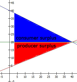
Before the tax, the supply and demand curves looked like this:

Consumer surplus is the area below the demand curve, above the price, up to the total number of goods sold. The basic reasoning behind this is that the demand curve gives the willingness-to-pay for each good, which decreases as more goods are sold because of diminishing marginal utility. So what this curve is saying is that the first hour of work was worth $40 to the employer, but each following hour was worth a bit less, until the 10^th hour of work was only worth $35. Thus the first hour gave $40-$20 = $20 of surplus, while the 10^th hour only gave $35-$20 = $15 of surplus.

Producer surplus is the area above the supply curve, below the price, again up to the total number of goods sold. The reasoning is the same: If the first hour of work cost $5 worth of time but the 10^th hour cost $10 worth of time, the first hour provided $20-$5 = $15 in producer surplus, but the 10^th hour only provided $20-$10 = $10 in producer surplus.

Imagine drawing a little 1-pixel-wide line straight down from the demand curve to the price for each hour and then adding up all those little lines into the total area under the curve, and similarly drawing little 1-pixel-wide lines straight up from the supply curve.

The employer was paying $20 * 40 = $800 for an amount of work that they actually valued at $1200 (the total area under the demand curve up to 40 hours), so they benefit by $400. The worker was being paid $800 for an amount of work that they would have been willing to accept $480 to do (the total area under the supply curve up to 40 hours), so they benefit $320. The sum of these is the total surplus $720.

After the tax, the employer is paying $22.50 * 35 = $787.50, but for an amount of work that they only value at $1093.75, so their new surplus is only $306.25. The worker is receiving $18 * 35 = $630, for an amount of work they’d have been willing to accept $385 to do, so their new surplus is $245. Even when you add back in the government revenue of $4.50 * 35 = $157.50, the total surplus is still only $708.75. What happened to that extra $11.25 of value? It simply disappeared. It’s gone. That’s what we mean by “deadweight loss”. That’s why there is a downside to taxation.

How large the deadweight loss is depends on the precise shape of the supply and demand curves, specifically on how elastic they are. Remember that elasticity is the proportional change in the quantity sold relative to the change in price. If increasing the price 1% makes you want to buy 2% less, you have a demand elasticity of -2. (Some would just say “2”, but then how do we say it if raising the price makes you want to buy more? The Law of Demand is more like what you’d call a guideline.) If increasing the price 1% makes you want to sell 0.5% more, you have a supply elasticity of 0.5.

If supply and demand are highly elastic, deadweight loss will be large, because even a small tax causes people to stop buying and selling a large amount of goods. If either supply or demand is inelastic, deadweight loss will be small, because people will more or less buy and sell as they always did regardless of the tax.

I’ve filled in the deadweight loss with brown in each of these graphs. They are designed to have the same tax rate, and the same price and quantity sold before the tax.

When supply and demand are elastic, the deadweight loss is large:

But when supply and demand are inelastic, the deadweight loss is small:

Notice that despite the original price and the tax rate being the same, the tax revenue is also larger in the case of inelastic supply and demand. (The total surplus is also larger, but it’s generally thought that we don’t have much control over the real value and cost of goods, so we can’t generally make something more inelastic in order to increase total surplus.)

Thus, all other things equal, it is better to tax goods that are inelastic, because this will raise more tax revenue while producing less deadweight loss.

But that’s not all that elasticity does!

At last, the end of our journey approaches: In the next post in this series, I will explain how elasticity affects who actually ends up bearing the burden of the tax.