How much should we give?

Nov 4 JDN 2458427

How much should we give of ourselves to others?

I’ve previously struggled with this basic question when it comes to donating money; I have written multiple posts on it now, some philosophical, some empirical, and some purely mathematical.

But the question is broader than this: We don’t simply give money. We also give effort. We also give emotion. Above all, we also give time. How much should we be volunteering? How many protest marches should we join? How many Senators should we call?

It’s easy to convince yourself that you aren’t doing enough. You can always point to some hour when you weren’t doing anything particularly important, and think about all the millions of lives that hang in the balance on issues like poverty and climate change, and then feel a wave of guilt for spending that hour watching Netflix or playing video games instead of doing one more march. This, however, is clearly unhealthy: You won’t actually make yourself into a more effective activist, you’ll just destroy yourself psychologically and become no use to anybody.

I previously argued for a sort of Kantian notion that we should commit to giving our fair share, defined as the amount we would have to give if everyone gave that amount. This is quite appealing, and if I can indeed get anyone to donate 1% of their income as a result, I will be quite glad. (If I can get 100 people to do so, that’s better than I could ever have done myself—a good example of highly cost-effective slacktivism.)

Lately I have come to believe that this is probably inadequate. We know that not everyone will take this advice, which means that by construction it won’t be good enough to actually solve global problems.

This means I must make a slightly greater demand: Define your fair share as the amount you would have to give if everyone among people who are likely to give gave that amount.

Unfortunately, this question is considerably harder. It may not even have a unique answer. The number of people willing to give an amount n is obviously dependent upon the amount x itself, and we are nowhere close to knowing what that function n(x) looks like.

So let me instead put some mathematical constraints on it, by choosing an elasticity. Instead of an elasticity of demand or elasticity of supply, we could call this an elasticity of contribution.

Presumably the elasticity is negative: The more you ask of people, the fewer people you’ll get to contribute.

Suppose that the elasticity is something like -0.5, where contribution is relatively inelastic. This means that if you increase the amount you ask for by 2%, you’ll only decrease the number of contributors by 1%. In that case, you should be like Peter Singer and ask for everything. At that point, you’re basically counting on Bill Gates to save us, because nobody else is giving anything. The total amount contributed n(x) * x is increasing in x.

On the other hand, suppose that elasticity is something like 2, where contribution is relatively elastic. This means that if you increase the amount you ask for by 2%, you will decrease the number of contributors by 4%. In that case, you should ask for very little. You’re asking everyone in the world to give 1% of their income, as I did earlier. The total amount contributed n(x) * x is now decreasing in x.

But there is also a third option: What if the elasticity is exactly -1, unit elastic? Then if you increase the amount you ask for by 2%, you’ll decrease the number of contributors by 2%. Then it doesn’t matter how much you ask for: The total amount contributed n(x) * x is constant.

Of course, there’s no guarantee that the elasticity is constant over all possible choices of x—indeed, it would be quite surprising if it were. A quite likely scenario is that contribution is inelastic for small amounts, then passes through a regime where it is nearly unit elastic, and finally it becomes elastic as you start asking for really large amounts of money.

The simplest way to model that is to just assume that n(x) is linear in x, something like n = N – k x.

There is a parameter N that sets the maximum number of people who will ever donate, and a parameter k that sets how rapidly the number of contributors drops off as the amount asked for increases.

The first-order condition for maximizing n(x) * x is then quite simple: x = N/(2k)

This actually turns out to be the precisely the point at which the elasticity of contribution is -1.

The total amount you can get under that condition is N2/(4k)

Of course, I have no idea what N and k are in real life, so this isn’t terribly helpful. But what I really want to know is whether we should be asking for more money from each person, or asking for less money and trying to get more people on board.

In real life we can sometimes do both: Ask each person to give more than they are presently giving, whatever they are presently giving. (Just be sure to run your slogans by a diverse committee, so you don’t end up with “I’ve upped my standards. Now, up yours!”) But since we’re trying to find a benchmark level to demand of ourselves, let’s ignore that for now.

About 25% of American adults volunteer some of their time, averaging 140 hours of volunteer work per year. This is about 1.6% of all the hours in a year, or 2.4% of all waking hours. Total monetary contributions in the US reached $400 billion for the first time this year; this is about 2.0% of GDP. So the balance between volunteer hours and donations is actually pretty even. It would probably be better to tilt it a bit more toward donations, but it’s really not bad. About 60% of US households made some sort of charitable contribution, though only half of these received the charitable tax deduction.

This suggests to me that the quantity of people who give is probably about as high as it’s going to get—and therefore we need to start talking more about the amount of money. We may be in the inelastic regime, where the way to increase total contributions is to demand more from each individual.

Our goal is to increase the total contribution to poverty eradication by about 1% of GDP in both the US and Europe. So if 60% of people give, and currently total contributions are about 2.0% of GDP, this means that the average contribution is about 3.3% of the contributor’s gross income. Therefore I should tell them to donate 4.3%, right? Not quite; some of them might drop out entirely, and the rest will have to give more to compensate.
Without knowing the exact form of the function n(x), I can’t say precisely what the optimal value is. But it is most likely somewhat larger than 4.3%; 5% would be a nice round number in the right general range. This would raise contributions in the US to 2.6% of GDP, or about $500 billion. That’s a 20% increase over the current level, which is large, but feasible.

Accomplishing a similar increase in Europe would then give us a total of $200 billion per year in additional funds to fight global poverty; this might not quite be enough to end world hunger (depending on which estimate you use), but it would definitely have a large impact.

I asked you before to give 1%. I am afraid I must now ask for more. Set a target of 5%. You don’t have to reach it this year; you can gradually increase your donations each year for several years (I call this “Save More Lives Tomorrow”, after Thaler’s highly successful program “Save More Tomorrow”). This is in some sense more than your fair share; I’m relying on the assumption that half the population won’t actually give anything. But ultimately this isn’t about what’s fair to us. It’s about solving global problems.

How not to do financial transaction tax

JDN 2457520

I strongly support the implementation of a financial transaction tax; like a basic income, it’s one of those economic policy ideas that are so brilliantly simple it’s honestly a little hard to believe how incredibly effective they are at making the world a better place. You mean we might be able to end stock market crashes just by implementing this little tax that most people will never even notice, and it will raise enough revenue to pay for food stamps? Yes, a financial transaction tax is that good.

So, keep that in mind when I say this:

TruthOut’s proposal for a financial transaction tax is somewhere between completely economically illiterate and outright insane.

They propose a 10% transaction tax on stocks and a 1% transaction tax on notional value of derivatives, then offer a “compromise” of 5% on stocks and 0.5% on derivatives. They make a bunch of revenue projections based on these that clearly amount to nothing but multiplying the current amount of transactions by the tax rate, which is so completely wrong we now officially have a left-wing counterpart to trickle-down voodoo economics.

Their argument is basically like this (I’m paraphrasing): “If we have to pay 5% sales tax on groceries, why shouldn’t you have to pay 5% on stocks?”

But that’s not how any of this works.

Demand for most groceries is very inelastic, especially in the aggregate. While you might change which groceries you’ll buy depending on their respective prices, and you may buy in bulk or wait for sales, over a reasonably long period (say a year) across a large population (say all of Michigan or all of the US), total amount of spending on groceries is extremely stable. People only need a certain amount of food, and they generally buy that amount and then stop.

So, if you implement a 5% sales tax that applies to groceries (actually sales tax in most states doesn’t apply to most groceries, but honestly it probably should—offset the regressiveness by providing more social services), people would just… spend about 5% more on groceries. Probably a bit less than that, actually, since suppliers would absorb some of the tax; but demand is much less elastic for groceries than supply, so buyers would bear most of the incidence of the tax. (It does not matter how the tax is collected; see my tax incidence series for further explanation of why.)

Other goods like clothing and electronics are a bit more elastic, so you’d get some deadweight loss from the sales tax; but at a typical 5% to 10% in the US this is pretty minimal, and even the hefty 20% or 30% VATs in some European countries only have a moderate effect. (Denmark’s 180% sales tax on cars seems a bit excessive to me, but it is Pigovian to disincentivize driving, so it also has very little deadweight loss.)

But what would happen if you implemented a 5% transaction tax on stocks? The entire stock market would immediately collapse.

A typical return on stocks is between 5% and 15% per year. As a rule of thumb, let’s say about 10%.

If you pay 5% sales tax and trade once per year, tax just cut your return in half.

If you pay 5% sales tax and trade twice per year, tax destroyed your return completely.

Even if you only trade once every five years, a 5% sales tax means that instead of your stocks being worth 61% more after those 5 years they are only worth 53% more. Your annual return has been reduced from 10% to 8.9%.

But in fact there are many perfectly legitimate reasons to trade as often as monthly, and a 5% tax would make monthly trading completely unviable.

Even if you could somehow stop everyone from pulling out all their money just before the tax takes effect, you would still completely dry up the stock market as a source of funding for all but the most long-term projects. Corporations would either need to finance their entire operations out of cash or bonds, or collapse and trigger a global depression.

Derivatives are even more extreme. The notional value of derivatives is often ludicrously huge; we currently have over a quadrillion dollars in notional value of outstanding derivatives. Assume that say 10% of those are traded every year, and we’re talking $100 trillion in notional value of transactions. At 0.5% you’re trying to take in a tax of $500 billion. That sounds fantastic—so much money!—but in fact what you should be thinking about is that’s a really strong avoidance incentive. You don’t think banks will find a way to restructure their trading practices—or stop trading altogether—to avoid this tax?

Honestly, maybe a total end to derivatives trading would be tolerable. I certainly think we need to dramatically reduce the amount of derivatives trading, and much of what is being traded—credit default swaps, collateralized debt obligations, synthetic collateralized debt obligations, etc.—really should not exist and serves no real function except to obscure fraud and speculation. (Credit default swaps are basically insurance you can buy on other people’s companies. There’s a reason you’re not allowed to buy insurance on other people’s stuff!) Interest rate swaps aren’t terrible (when they’re not being used to perpetrate the largest white-collar crime in history), but they also aren’t necessary. You might be able to convince me that commodity futures and stock options are genuinely useful, though even these are clearly overrated. (Fun fact: Futures markets have been causing financial crises since at least Classical Rome.) Exchange-traded funds are technically derivatives, and they’re just fine (actually ETFs are very low-risk, because they are inherently diversified—which is why you should probably be buying them); but actually their returns are more like stocks, so the 0.5% might not be insanely high in that case.

But stocks? We kind of need those. Equity financing has been the foundation of capitalism since the very beginning. Maybe we could conceivably go to a fully debt-financed system, but it would be a radical overhaul of our entire financial system and is certainly not something to be done lightly.

Indeed, TruthOut even seems to think we could apply the same sales tax rate to bonds, which means that debt financing would also collapse, and now we’re definitely talking about global depression. How exactly is anyone supposed to finance new investments, if they can’t sell stock or bonds? And a 5% tax on the face value of stock or bonds, for all practical purposes, is saying that you can’t sell stock or bonds. It would make no one want to buy them.

Wealthy investors buying of stocks and bonds is essentially no different than average folks buying food, clothing or other real “goods and services.”

Yes it is. It is fundamentally different.

People buy goods to use them. People buy stocks to make money selling them.

This seems perfectly obvious, but it is a vital distinction that seems to be lost on TruthOut.

When you buy an apple or a shoe or a phone or a car, you care how much it costs relative to how useful it is to you; if we make it a bit more expensive, that will make you a bit less likely to buy it—but probably not even one-to-one so that a 5% tax would reduce purchases by 5%; it would probably be more like a 2% reduction. Demand for goods is inelastic. Taxing them will raise a lot of revenue and not reduce the quantity purchased very much.

But when you buy a stock or a bond or an interest rate swap, you care how much it costs relative to what you will be able to sell it for—you care about not its utility but its return. So a 5% tax will reduce the amount of buying and selling by substantially more than 5%—it could well be 50% or even 100%. Demand for financial assets is elastic. Taxing them will not raise much revenue but will substantially reduce the quantity purchased.

Now, for some financial assets, we want to reduce the quantity purchased—the derivatives market is clearly too big, and high-frequency trading that trades thousands of times per second can do nothing but destabilize the financial system. Joseph Stiglitz supports a small financial transaction tax precisely because it would substantially reduce high-frequency trading, and he’s a Nobel Laureate as you may recall. Naturally, he was excluded from the SEC hearings on the subject, because reasons. But the figures Stiglitz is talking about (and I agree with) are on the order of 0.1% for stocks and 0.01% for derivatives—50 times smaller than what TruthOut is advocating.

At the end, they offer another “compromise”:

Okay, half it again, to a 2.5 percent tax on stocks and bonds and a 0.25 percent on derivative trades. That certainly won’t discourage stock and bond trading by the rich (not that that is an all bad idea either).

Yes it will. By a lot. That’s the whole point.

A financial transaction tax is a great idea whose time has come; let’s not ruin its reputation by setting it at a preposterous value. Just as a $15 minimum wage is probably a good idea but a $250 minimum wage is definitely a terrible idea, a 0.1% financial transaction tax could be very beneficial but a 5% financial transaction tax would clearly be disastrous.

Tax incidence revisited, part 5: Who really pays the tax?

JDN 2457359

I think all the pieces are now in place to really talk about tax incidence.

In earlier posts I discussed how taxes have important downsides, then talked about how taxes can distort prices, then explained that taxes are actually what gives money its value. In the most recent post in the series, I used supply and demand curves to show precisely how taxes create deadweight loss.

Now at last I can get to the fundamental question: Who really pays the tax?

The common-sense answer would be that whoever writes the check to the government pays the tax, but this is almost completely wrong. It is right about one aspect, a sort of political economy notion, which is that if there is any trouble collecting the tax, it’s generally that person who is on the hook to pay it. But especially in First World countries, most taxes are collected successfully almost all the time. Tax avoidance—using loopholes to reduce your tax burden—is all over the place, but tax evasion—illegally refusing to pay the tax you owe—is quite rare. And for this political economy argument to hold, you really need significant amounts of tax evasion and enforcement against it.

The real economic answer is that the person who pays the tax is the person who bears the loss in surplus. In essence, the person who bears the tax is the person who is most unhappy about it.

In the previous post in this series, I explained what surplus is, but it bears a brief repetition. Surplus is the value you get from purchases you make, in excess of the price you paid to get them. It’s measured in dollars, because that way we can read it right off the supply and demand curve. We should actually be adjusting for marginal utility of wealth and measuring in QALY, but that’s a lot harder so it rarely gets done.

In the graphs I drew in part 4, I already talked about how the deadweight loss is much greater if supply and demand are elastic than if they are inelastic. But in those graphs I intentionally set it up so that the elasticities of supply and demand were about the same. What if they aren’t?

Consider what happens if supply is very inelastic, but demand is very elastic. In fact, to keep it simple, lets suppose that supply is perfectly inelastic, but demand is perfectly elastic. This means that supply elasticity is 0, but demand elasticity is infinite.

The zero supply elasticity means that the worker would actually be willing to work up to their maximum hours for nothing, but is unwilling to go above that regardless of the wage. They have a specific amount of hours they want to work, regardless of what they are paid.

The infinite demand elasticity means that each hour of work is worth exactly the same amount the employer, with no diminishing returns. They have a specific wage they are willing to pay, regardless of how many hours it buys.

Both of these are quite extreme; it’s unlikely that in real life we would ever have an elasticity that is literally zero or infinity. But we do actually see elasticities that get very low or very high, and qualitatively they act the same way.

So let’s suppose as before that the wage is $20 and the number of hours worked is 40. The supply and demand graph actually looks a little weird: There is no consumer surplus whatsoever.

incidence_infinite_notax_surplus

Each hour is worth $20 to the employer, and that is what they shall pay. The whole graph is full of producer surplus; the worker would have been willing to work for free, but instead gets $20 per hour for 40 hours, so they gain a whopping $800 in surplus.

incidence_infinite_tax_surplus

Now let’s implement a tax, say 50% to make it easy. (That’s actually a huge payroll tax, and if anybody ever suggested implementing that I’d be among the people pulling out a Laffer curve to show them why it’s a bad idea.)

Normally a tax would push the demand wage higher, but in this case $20 is exactly what they can afford, so they continue to pay exactly the same as if nothing had happened. This is the extreme example in which your “pre-tax” wage is actually your pre-tax wage, what you’d get if there hadn’t been a tax. This is the only such example—if demand elasticity is anything less than infinity, the wage you see listed as “pre-tax” will in fact be higher than what you’d have gotten in the absence of the tax.

The tax revenue is therefore borne entirely by the worker; they used to take home $20 per hour, but now they only get $10. Their new surplus is only $400, precisely 40% lower. The extra $400 goes directly to the government, which makes this example unusual in another way: There is no deadweight loss. The employer is completely unaffected; their surplus goes from zero to zero. No surplus is destroyed, only moved. Surplus is simply redistributed from the worker to the government, so the worker bears the entirety of the tax. Note that this is true regardless of who actually writes the check; I didn’t even have to include that in the model. Once we know that there was a tax imposed on each hour of work, the market prices decided who would bear the burden of that tax.

By Jove, we’ve actually found an example in which it’s fair to say “the government is taking my hard-earned money!” (I’m fairly certain if you replied to such people with “So you think your supply elasticity is zero but your employer’s demand elasticity is infinite?” you would be met with blank stares or worse.)

This is however quite an extreme case. Let’s try a more realistic example, where supply elasticity is very small, but not zero, and demand elasticity is very high, but not infinite. I’ve made the demand elasticity -10 and the supply elasticity 0.5 for this example.

incidence_supply_notax_surplus

Before the tax, the wage was $20 for 40 hours of work. The worker received a producer surplus of $700. The employer received a consumer surplus of only $80. The reason their demand is so elastic is that they are only barely getting more from each hour of work than they have to pay.

Total surplus is $780.

incidence_supply_tax_surplus

After the tax, the number of hours worked has dropped to 35. The “pre-tax” (demand) wage has only risen to $20.25. The after-tax (supply) wage the worker actually receives has dropped all the way to $10. The employer’s surplus has only fallen to $65.63, a decrease of $14.37 or 18%. Meanwhile the worker’s surplus has fallen all the way to $325, a decrease of $275 or 46%. The employer does feel the tax, but in both absolute and relative terms, the worker feels the tax much more than the employer does.

The tax revenue is $358.75, which means that the total surplus has been reduced to $749.38. There is now $30.62 of deadweight loss. Where both elasticities are finite and nonzero, deadweight loss is basically inevitable.

In this more realistic example, the burden was shared somewhat, but it still mostly fell on the worker, because the worker had a much lower elasticity. Let’s try turning the tables and making demand elasticity low while supply elasticity is high—in fact, once again let’s illustrate by using the extreme case of zero versus infinity.

In order to do this, I need to also set a maximum wage the employer is willing to pay. With nonzero elasticity, that maximum sort of came out automatically when the demand curve hits zero; but when elasticity is zero, the line is parallel so it never crosses. Let’s say in this case that the maximum is $50 per hour.

(Think about why we didn’t need to set a minimum wage for the worker when supply was perfectly inelastic—there already was a minimum, zero.)

incidence_infinite2_notax_surplus

This graph looks deceptively similar to the previous; basically all that has happened is the supply and demand curves have switched places, but that makes all the difference. Now instead of the worker getting all the surplus, it’s the employer who gets all the surplus. At their maximum wage of $50, they are getting $1200 in surplus.

Now let’s impose that same 50% tax again.

incidence_infinite2_tax_surplus

The worker will not accept any wage less than $20, so the demand wage must rise all the way to $40. The government will then receive $800 in revenue, while the employer will only get $400 in surplus. Notice again that the deadweight loss is zero. The employer will now bear the entire burden of the tax.

In this case the “pre-tax” wage is basically meaningless; regardless of the value of the tax the worker would receive the same amount, and the “pre-tax” wage is really just an accounting mechanism the government uses to say how large the tax is. They could just as well have said, “Hey employer, give us $800!” and the outcome would be the same. This is called a lump-sum tax, and they don’t work in the real world but are sometimes used for comparison. The thing about a lump-sum tax is that it doesn’t distort prices in any way, so in principle you could use it to redistribute wealth however you want. But in practice, there’s no way to implement a lump-sum tax that would be large enough to raise sufficient revenue but small enough to be affordable by the entire population. Also, a lump-sum tax is extremely regressive, hurting the poor tremendously while the rich feel nothing. (Actually the closest I can think of to a realistic lump-sum tax would be a basic income, which is essentially a negative lump-sum tax.)

I could keep going with more examples, but the basic argument is the same.

In general what you will find is that the person who bears a tax is the person who has the most to lose if less of that good is sold. This will mean their supply or demand is very inelastic and their surplus is very large.

Inversely, the person who doesn’t feel the tax is the person who has the least to lose if the good stops being sold. That will mean their supply or demand is very elastic and their surplus is very small.
Once again, it really does not matter how the tax is collected. It could be taken entirely from the employer, or entirely from the worker, or shared 50-50, or 60-40, or whatever. As long as it actually does get paid, the person who will actually feel the tax depends upon the structure of the market, not the method of tax collection. Raising “employer contributions” to payroll taxes won’t actually make workers take any more home; their “pre-tax” wages will simply be adjusted downward to compensate. Likewise, raising the “employee contribution” won’t actually put more money in the pockets of the corporation, it will just force them to raise wages to avoid losing employees. The actual amount that each party must contribute to the tax isn’t based on how the checks are written; it’s based on the elasticities of the supply and demand curves.

And that’s why I actually can’t get that strongly behind corporate taxes; even though they are formally collected from the corporation, they could simply be hurting customers or employees. We don’t actually know; we really don’t understand the incidence of corporate taxes. I’d much rather use income taxes or even sales taxes, because we understand the incidence of those.

Tax incidence revisited, part 4: Surplus and deadweight loss

JDN 2457355

I’ve already mentioned the fact that taxation creates deadweight loss, but in order to understand tax incidence it’s important to appreciate exactly how this works.

Deadweight loss is usually measured in terms of total economic surplus, which is a strange and deeply-flawed measure of value but relatively easy to calculate.

Surplus is based upon the concept of willingness-to-pay; the value of something is determined by the maximum amount of money you would be willing to pay for it.

This is bizarre for a number of reasons, and I think the most important one is that people differ in how much wealth they have, and therefore in their marginal utility of wealth. $1 is worth more to a starving child in Ghana than it is to me, and worth more to me than it is to a hedge fund manager, and worth more to a hedge fund manager than it is to Bill Gates. So when you try to set what something is worth based on how much someone will pay for it, which someone are you using?

People also vary, of course, in how much real value a good has to them: Some people like dark chocolate, some don’t. Some people love spicy foods and others despise them. Some people enjoy watching sports, others would rather read a book. A meal is worth a lot more to you if you haven’t eaten in days than if you just ate half an hour ago. That’s not actually a problem; part of the point of a market economy is to distribute goods to those who value them most. But willingness-to-pay is really the product of two different effects: The real effect, how much utility the good provides you; and the wealth effect, how your level of wealth affects how much you’d pay to get the same amount of utility. By itself, willingness-to-pay has no means of distinguishing these two effects, and actually I think one of the deepest problems with capitalism is that ultimately capitalism has no means of distinguishing these two effects. Products will be sold to the highest bidder, not the person who needs it the most—and that’s why Americans throw away enough food to end world hunger.

But for today, let’s set that aside. Let’s pretend that willingness-to-pay is really a good measure of value. One thing that is really nice about it is that you can read it right off the supply and demand curves.

When you buy something, your consumer surplus is the difference between your willingness-to-pay and how much you actually did pay. If a sandwich is worth $10 to you and you pay $5 to get it, you have received $5 of consumer surplus.

When you sell something, your producer surplus is the difference between how much you were paid and your willingness-to-accept, which is the minimum amount of money you would accept to part with it. If making that sandwich cost you $2 to buy ingredients and $1 worth of your time, your willingness-to-accept would be $3; if you then sell it for $5, you have received $2 of producer surplus.

Total economic surplus is simply the sum of consumer surplus and producer surplus. One of the goals of an efficient market is to maximize total economic surplus.

Let’s return to our previous example, where a 20% tax raised the original wage from $22.50 and thus resulted in an after-tax wage of $18.

Before the tax, the supply and demand curves looked like this:

equilibrium_notax

Consumer surplus is the area below the demand curve, above the price, up to the total number of goods sold. The basic reasoning behind this is that the demand curve gives the willingness-to-pay for each good, which decreases as more goods are sold because of diminishing marginal utility. So what this curve is saying is that the first hour of work was worth $40 to the employer, but each following hour was worth a bit less, until the 10th hour of work was only worth $35. Thus the first hour gave $40-$20 = $20 of surplus, while the 10th hour only gave $35-$20 = $15 of surplus.

Producer surplus is the area above the supply curve, below the price, again up to the total number of goods sold. The reasoning is the same: If the first hour of work cost $5 worth of time but the 10th hour cost $10 worth of time, the first hour provided $20-$5 = $15 in producer surplus, but the 10th hour only provided $20-$10 = $10 in producer surplus.

Imagine drawing a little 1-pixel-wide line straight down from the demand curve to the price for each hour and then adding up all those little lines into the total area under the curve, and similarly drawing little 1-pixel-wide lines straight up from the supply curve.

surplus

The employer was paying $20 * 40 = $800 for an amount of work that they actually valued at $1200 (the total area under the demand curve up to 40 hours), so they benefit by $400. The worker was being paid $800 for an amount of work that they would have been willing to accept $480 to do (the total area under the supply curve up to 40 hours), so they benefit $320. The sum of these is the total surplus $720.

equilibrium_notax_surplus

After the tax, the employer is paying $22.50 * 35 = $787.50, but for an amount of work that they only value at $1093.75, so their new surplus is only $306.25. The worker is receiving $18 * 35 = $630, for an amount of work they’d have been willing to accept $385 to do, so their new surplus is $245. Even when you add back in the government revenue of $4.50 * 35 = $157.50, the total surplus is still only $708.75. What happened to that extra $11.25 of value? It simply disappeared. It’s gone. That’s what we mean by “deadweight loss”. That’s why there is a downside to taxation.

equilibrium_tax_surplus

How large the deadweight loss is depends on the precise shape of the supply and demand curves, specifically on how elastic they are. Remember that elasticity is the proportional change in the quantity sold relative to the change in price. If increasing the price 1% makes you want to buy 2% less, you have a demand elasticity of -2. (Some would just say “2”, but then how do we say it if raising the price makes you want to buy more? The Law of Demand is more like what you’d call a guideline.) If increasing the price 1% makes you want to sell 0.5% more, you have a supply elasticity of 0.5.

If supply and demand are highly elastic, deadweight loss will be large, because even a small tax causes people to stop buying and selling a large amount of goods. If either supply or demand is inelastic, deadweight loss will be small, because people will more or less buy and sell as they always did regardless of the tax.

I’ve filled in the deadweight loss with brown in each of these graphs. They are designed to have the same tax rate, and the same price and quantity sold before the tax.

When supply and demand are elastic, the deadweight loss is large:

equilibrium_elastic_tax_surplus

But when supply and demand are inelastic, the deadweight loss is small:

equilibrium_inelastic_tax_surplus

Notice that despite the original price and the tax rate being the same, the tax revenue is also larger in the case of inelastic supply and demand. (The total surplus is also larger, but it’s generally thought that we don’t have much control over the real value and cost of goods, so we can’t generally make something more inelastic in order to increase total surplus.)

Thus, all other things equal, it is better to tax goods that are inelastic, because this will raise more tax revenue while producing less deadweight loss.

But that’s not all that elasticity does!

At last, the end of our journey approaches: In the next post in this series, I will explain how elasticity affects who actually ends up bearing the burden of the tax.

Elasticity and the Law of Supply

JDN 2457292 EDT 16:16.

Today’s post is kind of a mirror image of the previous post earlier this week; I was talking about demand before, and now I’m talking about supply. (In the next post, I’ll talk about how the two work together to determine the actual price of goods.)

Just as there is an elasticity of demand which describes how rapidly the quantity demanded changes with changes in price, likewise there is an elasticity of supply which describes how much the quantity supplied changes with changes in price.

The elasticity of supply is defined as the proportional change in quantity supplied divided by the proportional change in price; so for example if the number of cars produced increases 10% when the price of cars increases by 5%, the elasticity of supply of cars would be 10%/5% = 2.

Goods that have high elasticity of supply will rapidly flood the market if the price increases even a small amount; goods that have low elasticity of supply will sell at about the same rate as ever even if the price increases dramatically.

Generally, the more initial investment of capital a good requires, the lower its elasticity of supply is going to be.

If most of the cost of production is in the actual marginal cost of producing each new gizmo, then elasticity of supply will be high, because it’s easy to produce more or produce less as the market changes.

But if most of the cost is in building machines or inventing technologies or training employees which already has to be done in order to make any at all, while the cost of each individual gizmo is unimportant, the elasticity of supply will be low, because there’s no sense letting all that capital you invested go to waste.
We can see these differences in action by comparing different sources of electric power.

Photovoltaic solar power has a high elasticity of supply, because building new solar panels is cheap and fast. As the price of solar energy fluctuates, the amount of solar panel produced changes rapidly. Technically this is actually a “fixed capital” cost, but it’s so modular that you can install as little or as much solar power capacity as you like, which makes it behave a lot more like a variable cost than a fixed cost. As a result, a 1% increase in the price paid for solar power increases the amount supplied by a whopping 2.7%, a supply elasticity of 2.7.

Oil has a moderate elasticity of supply, because finding new oil reserves is expensive but feasible. A lot of oil in the US is produced by small wells; 18% of US oil is produced by wells that put out less than 10 barrels per day. Those small wells can be turned on and off as the price of oil changes, and new ones can be built if it becomes profitable. As a result, investment in oil production is very strongly correlated with oil prices. Still, overall production of oil changes only moderate amounts; in the US it had been steadily decreasing since 1970 until very recently when new technologies and weakened regulations resulted in a rapid increase to near-1970s levels. We sort of did hit peak oil; but it’s never quite that simple.

Nuclear fission has a very low elasticity of supply, because building a nuclear reactor is extremely expensive and requires highly advanced expertise. Building a nuclear power plant costs upward of $35 billion. Once a reactor is built, the cost of generating more power is relatively trivial; three-fourths of the cost a nuclear power plant will ever pay is paid simply to build it (or to pay back the debt incurred by doing so). Even if the price of uranium plummets or the price of oil skyrockets, it would take a long time before more nuclear power plants would be built in response.

Elasticity of supply is generally a lot larger in the long run than in the short run. Over a period of a few days or months, many types of production can’t be changed significantly. If you have a corn field, you grow as much corn as you can this season; even if the price rose substantially you couldn’t actually grow any more than your field will allow. But over a period of a year to a few years, most types of production can be changed; continuing with the corn example, you could buy new land to plant corn next season.

The Law of Supply is actually a lot closer to a true law than the Law of Demand. A negative elasticity of supply is almost unheard of; at worst elasticity of supply can sometimes drop close to zero. It really is true that elasticity of supply is almost always positive.

Land has an elasticity near zero; it’s extremely expensive (albeit not impossible; Singapore does it rather frequently) to actually create new land. As a result there’s really no good reason to ever raise the price of land; higher land prices don’t incentivize new production, they just transfer wealth to landowners. That’s why a land tax is such a good idea; it would transfer some of that wealth away from landowners and let us use it for public goods like infrastructure or research, or even just give it to the poor. A few countries actually have tried this; oddly enough, they include Singapore and Denmark, two of the few places in the world where the elasticity of land supply is appreciably above zero!

Real estate in general (which is what most property taxes are imposed on) is much trickier: In the short run it seems to have a very low elasticity, because building new houses or buildings takes a lot of time and money. But in the long run it actually has a high elasticity of supply, because there is a lot of profit to be made in building new structures if you can fund projects 10 or 15 years out. The short-run elasticity is something like 0.2, meaning a 1% increase in price only yields a 0.2% increase in supply; but the long-run elasticity may be as high as 8, meaning that a 1% increase in price yields an 8% increase in supply. This is why property taxes and rent controls seem like a really good idea at the time but actually probably have the effect of making housing more expensive. The economics of real estate has a number of fundamental differences from the economics of most other goods.

Many important policy questions ultimately hinge upon the elasticity of supply: If elasticity is high, then taxing or regulating something is likely to cause large distortions of the economy, while if elasticity is low, taxes and regulations can be used to support public goods or redistribute wealth without significant distortion to the economy. On the other hand, if elasticity is high, markets generally function well on their own, while if elasticity is low, prices can get far out of whack. As a general rule of thumb, government intervention in markets is most useful and most necessary when elasticity is low.

Elasticity and the Law of Demand

JDN 2457289 EDT 21:04

This will be the second post in my new bite-size format, the first one that’s in the middle of the week.

I’ve alluded previously to the subject of demand elasticity, but I think it’s worth explaining in a little more detail. The basic concept is fairly straightforward: Demand is more elastic when the amount that people want to buy changes a large amount for a small change in price. The opposite is inelastic.

Apples are a relatively elastic good. If the price of apples goes up, people buy fewer apples. Maybe they buy other fruit instead, such as oranges or bananas; or maybe they give up on fruit and eat something else, like rice.

Salt is an extremely inelastic good. No matter what the price of salt is, at least within the range it has been for the last few centuries, people are going to continue to buy pretty much the same amount of salt. (In ancient times salt was actually expensive enough that people couldn’t afford enough of it, which was particularly harmful in desert regions. Mark Kulansky’s book Salt on this subject is surprisingly compelling, given the topic.)
Specifically, the elasticity is equal to the proportional change in quantity demanded, divided by the proportional change in price.

For example, if the price of gas rises from $2 per gallon to $3 per gallon, that’s a 50% increase. If the quantity of gas purchase then falls from 100 billion gallons to 90 billion gallons, that’s a 10% decrease. If increasing the price by 50% decreased the quantity demanded by 10%, that would be a demand elasticity of -10%/50% = -1/5 = -0.2

In practice, measuring elasticity is more complicated than that, because supply and demand are both changing at the same time; so when we see a price change and a quantity change, it isn’t always clear how much of each change is due to supply and how much is due to demand. Sophisticated econometric techniques have been developed to try to separate these two effects (in future posts I plan to explain the basics of some of these techniques), but it’s difficult and not always successful.

In general, markets function better when supply and demand are more elastic. When shifts in price trigger large shifts in quantity, this creates pressure on the price to remain at a fixed level rather than jumping up and down. This in turn means that the market will generally be predictable and stable.

It’s also much harder to make monopoly profits in a market with elastic demand; even if you do have a monopoly, if demand is highly elastic then raising the price won’t make you any money, because whatever you gain in selling each gizmo for more, you’ll lose in selling fewer gizmos. In fact, the profit margin for a monopoly is inversely proportional to the elasticity of demand.

Markets do not function well when supply and demand are highly inelastic. Monopolies can become very powerful and result in very large losses of human welfare. A particularly vivid example of this was in the news recently, when a company named Turing purchased the rights to a drug called Daraprim used primarily by AIDS patients, then hiked the price from $13.50 to $750. This made enough people mad that the CEO has since promised to bring it back down, though he hasn’t said how far.

That price change was only possible because Daraprim has highly inelastic demand—if you’ve got AIDS, you’re going to take AIDS medicine, as much as prescribed, provided only that it doesn’t drive you completely bankrupt. (Not an unreasonable fear, as medical costs are the leading cause of bankruptcy in the United States.) This raised price probably would bankrupt a few people, but for the most part it wouldn’t affect the amount of drug sold; it would just funnel a huge amount of money from AIDS patients to the company. This is probably part of why it made people so mad; that and there would probably be a few people who died because they couldn’t afford this new expensive medication.

Imagine if a company had tried to pull the same stunt for a more elastic good, like apples. “CEO buys up all apple farms, raises price of apples from $2 per pound to $100 per pound.” What’s going to happen then? People are not going to buy any apples. Perhaps a handful of the most die-hard apple lovers still would, but the rest of us are going to meet our fruit needs elsewhere.

For most goods most of the time, elasticity of demand is negative, meaning that as price increases, quantity demanded decreases. This is in fact called the Law of Demand; but as I’ve said, “laws” in economics are like the Pirate Code: They’re really more what you’d call “guidelines”.
There are three major exceptions to the Law of Demand. The first one is the one most economists talk about, and it almost never happens. The second one is talked about occasionally, and it’s quite common. The third one is almost never talked about, and yet it is by far the most common and one of the central driving forces in modern capitalism.
The exception that we usually talk about in economics is called the Giffen Effect. A Giffen good is a good that’s so cheap and such a bare necessity that when it becomes more expensive, you won’t be able to buy less of it; instead you’ll buy more of it, and buy less of other things with your reduced income.

It’s very hard to come up with empirical examples of Giffen goods, but it’s an easy theoretical argument to make. Suppose you’re buying grapes for a party, and you know you need 4 bags of grapes. You have $10 to spend. Suppose there are green grapes selling for $1 per bag and red grapes selling for $4 per bag, and suppose you like red grapes better. With your $10, you can buy 2 bags of green grapes and 2 bags of red grapes, and that’s the 4 bags you need. But now suppose that the price of green grapes rises to $2 per bag. In order to afford 4 bags of grapes, you now need to buy 3 bags of green grapes and only 1 bag of red grapes. Even though it was the price of green grapes that rose, you ended up buying more green grapes. In this scenario, green grapes are a Giffen good.

The exception that is talked about occasionally and occurs a lot in real life is the Veblen Effect. Whereas a Giffen good is a very cheap bare necessity, a Veblen good is a very expensive pure luxury.

The whole point of buying a Veblen good is to prove that you can. You don’t buy a Ferrari because a Ferrari is a particularly nice automobile (a Prius is probably better, and a Tesla certainly is); you buy a Ferrari to show off that you’re so rich you can buy a Ferrari.

On my previous post, jenszorn asked: “Much of consumer behavior is irrational by your standards. But people often like to spend money just for the sake of spending and for showing off. Why else does a Rolex carry a price tag for $10,000 for a Rolex watch when a $100 Seiko keeps better time and requires far less maintenance?” Veblen goods! It’s not strictly true that Veblen goods are irrational; it can be in any particular individual’s best interest is served by buying Veblen goods in order to signal their status and reap the benefits of that higher status. However, it’s definitely true that Veblen goods are inefficient; because ostentatious displays of wealth are a zero-sum game (it’s not about what you have, it’s about what you have that others don’t), any resources spent on rich people proving how rich they are are resources that society could otherwise have used, say, feeding the poor, curing diseases, building infrastructure, or colonizing other planets.

Veblen goods can also result in a violation of the Law of Demand, because raising the price of a Veblen good like Ferraris or Rolexes can make them even better at showing off how rich you are, and therefore more appealing to the kind of person who buys them. Conversely, lowering the price might not result in any more being purchased, because they wouldn’t seem as impressive anymore. Currently a Ferrari costs about $250,000; if they reduced that figure to $100,000, there aren’t a lot of people who would suddenly find it affordable, but many people who currently buy Ferraris might switch to Bugattis or Lamborghinis instead. There are limits to this, of course: If the price of a Ferrari dropped to $2,000, people wouldn’t buy them to show off anymore; but the far larger effect would be the millions of people buying them because you can now get a perfectly good car for $2,000. Yes, I would sell my dear little Smart if it meant I could buy a Ferrari instead and save $8,000 at the same time.

But the third major exception to the Law of Demand is actually the most important one, yet it’s the one that economists hardly ever talk about: Speculation.

The most common reason why people would buy more of something that has gotten more expensive is that they expect it to continue getting more expensive, and then they will be able to sell what they bought at an even higher price and make a profit.

When the price of Apple stock goes up, do people stop buying Apple stock? On the contrary, they almost certainly start buying more—and then the price goes up even further still. If rising prices get self-fulfilling enough, you get an asset bubble; it grows and grows until one day it can’t, and then the bubble bursts and prices collapse again. This has happened hundreds of times in history, from the Tulip Mania to the Beanie Baby Bubble to the Dotcom Boom to the US Housing Crisis.

It isn’t necessarily irrational to participate in a bubble; some people must be irrational, but most people can buy above what they would be willing to pay by accurately predicting that they’ll find someone else who is willing to pay an even higher price later. It’s called Greater Fool Theory: The price I paid may be foolish, but I’ll find someone who is even more foolish to take it off my hands. But like Veblen goods, speculation goods are most definitely inefficient; nothing good comes from prices that rise and fall wildly out of sync with the real value of goods.

Speculation goods are all around us, from stocks to gold to real estate. Most speculation goods also serve some other function (though some, like gold, are really mostly just Veblen goods otherwise; actual useful applications of gold are extremely rare), but their speculative function often controls their price in a way that dominates all other considerations. There’s no real limit to how high or low the price can go for a speculation good; no longer tied to the real value of the good, it simply becomes a question of how much people decide to pay.

Indeed, speculation bubbles are one of the fundamental problems with capitalism as we know it; they are one of the chief causes of the boom-and-bust business cycle that has cost the world trillions of dollars and thousands of lives. Most of our financial industry is now dedicated to the trading of speculation goods, and finance is taking over a larger and larger section of our economy all the time. Many of the world’s best and brightest are being funneled into finance instead of genuinely productive industries; 15% of Harvard grads take a job in finance, and almost half did just before the crash. The vast majority of what goes on in our financial system is simply elaborations on speculation; very little real productivity ever enters into the equation.

In fact, as a general rule I think when we see a violation of the Law of Demand, we know that something is wrong in the economy. If there are Giffen goods, some people are too poor to buy what they really need. If there are Veblen goods, inequality is too large and people are wasting resources competing for status. And since there are always speculation goods, the history of capitalism has been a history of market instability.

Fortunately, elasticity of demand is usually negative: As the price goes up, people want to buy less. How much less is the elasticity.

What you need to know about tax incidence

JDN 2457152 EDT 14:54.

I said in my previous post that I consider tax incidence to be one of the top ten things you should know about economics. If I actually try to make a top ten list, I think it goes something like this:

  1. Supply and demand
  2. Monopoly and oligopoly
  3. Externalities
  4. Tax incidence
  5. Utility, especially marginal utility of wealth
  6. Pareto-efficiency
  7. Risk and loss aversion
  8. Biases and heuristics, including sunk-cost fallacy, scope neglect, herd behavior, anchoring and representative heuristic
  9. Asymmetric information
  10. Winner-takes-all effect

So really tax incidence is in my top five things you should know about economics, and yet I still haven’t talked about it very much. Well, today I will. The basic principles of supply and demand I’m basically assuming you know, but I really should spend some more time on monopoly and externalities at some point.

Why is tax incidence so important? Because of one central fact: The person who pays the tax is not the person who writes the check.

It doesn’t matter whether a tax is paid by the buyer or the seller; it matters what the buyer and seller can do to avoid the tax. If you can change your behavior in order to avoid paying the tax—buy less stuff, or buy somewhere else, or deduct something—you will not bear the tax as much as someone else who can’t do anything to avoid the tax, even if you are the one who writes the check. If you can avoid it and they can’t, other parties in the transaction will adjust their prices in order to eat the tax on your behalf.

Thus, if you have a good that you absolutely must buy no matter what—like, say, table saltand then we make everyone who sells that good pay an extra $5 per kilogram, I can guarantee you that you will pay an extra $5 per kilogram, and the suppliers will make just as much money as they did before. (A salt tax would be an excellent way to redistribute wealth from ordinary people to corporations, if you’re into that sort of thing. Not that we have any trouble doing that in America.)

On the other hand, if you have a good that you’ll only buy at a very specific price—like, say, fast food—then we can make you write the check for a tax of an extra $5 per kilogram you use, and in real terms you’ll pay hardly any tax at all, because the sellers will either eat the cost themselves by lowering the prices or stop selling the product entirely. (A fast food tax might actually be a good idea as a public health measure, because it would reduce production and consumption of fast food—remember, heart disease is one of the leading causes of death in the United States, making cheeseburgers a good deal more dangerous than terrorists—but it’s a bad idea as a revenue measure, because rather than pay it, people are just going to buy and sell less.)

In the limit in which supply and demand are both completely fixed (perfectly inelastic), you can tax however you want and it’s just free redistribution of wealth however you like. In the limit in which supply and demand are both locked into a single price (perfectly elastic), you literally cannot tax that good—you’ll just eliminate production entirely. There aren’t a lot of perfectly elastic goods in the real world, but the closest I can think of is cash. If you instituted a 2% tax on all cash withdrawn, most people would stop using cash basically overnight. If you want a simple way to make all transactions digital, find a way to enforce a cash tax. When you have a perfect substitute available, taxation eliminates production entirely.

To really make sense out of tax incidence, I’m going to need a lot of a neoclassical economists’ favorite thing: Supply and demand curves. These things pop up everywhere in economics; and they’re quite useful. I’m not so sure about their application to things like aggregate demand and the business cycle, for example, but today I’m going to use them for the sort of microeconomic small-market stuff that they were originally designed for; and what I say here is going to be basically completely orthodox, right out of what you’d find in an ECON 301 textbook.

Let’s assume that things are linear, just to make the math easier. You’d get basically the same answers with nonlinear demand and supply functions, but it would be a lot more work. Likewise, I’m going to assume a unit tax on goods—like $2890 per hectare—as opposed to a proportional tax on sales—like 6% property tax—again, for mathematical simplicity.

The next concept I’m going to have to talk about is elasticitywhich is the proportional amount that quantity sold changes relative to price. If price increases 2% and you buy 4% less, you have a demand elasticity of -2. If price increases 2% and you buy 1% less, you have a demand elasticity of -1/2. If price increases 3% and you sell 6% more, you have a supply elasticity of 2. If price decreases 5% and you sell 1% less, you have a supply elasticity of 1/5.

Elasticity doesn’t have any units of measurement, it’s just a number—which is part of why we like to use it. It also has some very nice mathematical properties involving logarithms, but we won’t be needing those today.

The price that renters are willing and able to pay, the demand price PD will start at their maximum price, the reserve price PR, and then it will decrease linearly according to the quantity of land rented Q, according to a linear function (simply because we assumed that) which will vary according to a parameter e that represents the elasticity of demand (it isn’t strictly equal to it, but it’s sort of a linearization).

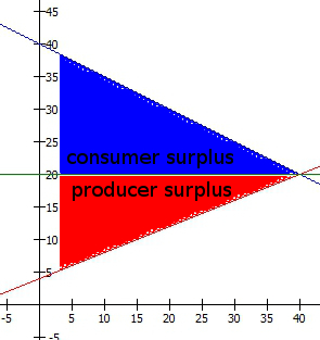
We’re interested in what is called the consumer surplus; it is equal to the total amount of value that buyers get from their purchases, converted into dollars, minus the amount they had to pay for those purchases. This we add to the producer surplus, which is the amount paid for those purchases minus the cost of producing themwhich is basically just the same thing as profit. Togerther the consumer surplus and producer surplus make the total economic surplus, which economists generally try to maximize. Because different people have different marginal utility of wealth, this is actually a really terrible idea for deep and fundamental reasons—taking a house from Mitt Romney and giving it to a homeless person would most definitely reduce economic surplus, even though it would obviously make the world a better place. Indeed, I think that many of the problems in the world, particularly those related to inequality, can be traced to the fact that markets maximize economic surplus rather than actual utility. But for now I’m going to ignore all that, and pretend that maximizing economic surplus is what we want to do.

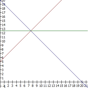
You can read off the economic surplus straight from the supply and demand curves; it’s the area between the lines. (Mathematically, it’s an integral; but that’s equivalent to the area under a curve, and with straight lines they’re just triangles.) I’m going to call the consumer surplus just “surplus”, and producer surplus I’ll call “profit”.

Below the demand curve and above the price is the surplus, and below the price and above the supply curve is the profit:

elastic_supply_competitive_labeled

I’m going to be bold here and actually use equations! Hopefully this won’t turn off too many readers. I will give each equation in both a simple text format and in proper LaTeX. Remember, you can render LaTeX here.

PD = PR – 1/e * Q

P_D = P_R – \frac{1}{e} Q \\

The marginal cost that landlords have to pay, the supply price PS, is a bit weirder, as I’ll talk about more in a moment. For now let’s say that it is a linear function, starting at zero cost for some quantity Q0 and then increases linearly according to a parameter n that similarly represents the elasticity of supply.

PS = 1/n * (Q – Q0)

P_S = \frac{1}{n} \left( Q – Q_0 \right) \\

Now, if you introduce a tax, there will be a difference between the price that renters pay and the price that landlords receive—namely, the tax, which we’ll call T. I’m going to assume that, on paper, the landlord pays the whole tax. As I said above, this literally does not matter. I could assume that on paper the renter pays the whole tax, and the real effect on the distribution of wealth would be identical. All we’d have to do is set PD = P and PS = P – T; the consumer and producer surplus would end up exactly the same. Or we could do something in between, with P’D = P + rT and P’S = P – (1 – r) T.

Then, if the market is competitive, we just set the prices equal, taking the tax into account:

P = PD – T = PR – 1/e * Q – T = PS = 1/n * (Q – Q0)

P= P_D – T = P_R – \frac{1}{e} Q – T= P_S = \frac{1}{n} \left(Q – Q_0 \right) \\

P_R – 1/e * Q – T = 1/n * (Q – Q0)

P_R – \frac{1}{e} Q – T = \frac{1}{n} \left(Q – Q_0 \right) \\

Notice the equivalency here; if we set P’D = P + rT and P’S = P – (1 – r) T, so that the consumer now pays a fraction of the tax r.

P = P’D – rT = P_r – 1/e*Q = P’S + (1 – r) T + 1/n * (Q – Q0) + (1 – r) T

P^\prime_D – r T = P = P_R – \frac{1}{e} Q = P^\prime_S = \frac{1}{n} \left(Q – Q_0 \right) + (1 – r) T\\

The result is exactly the same:

P_R – 1/e * Q – T = 1/n * (Q – Q0)

P_R – \frac{1}{e} Q – T = \frac{1}{n} \left(Q – Q_0 \right) \\

I’ll spare you the algebra, but this comes out to:

Q = (PR – T)/(1/n + 1/e) + (Q0)/(1 + n/e)

Q = \frac{P_R – T}{\frac{1}{n} + \frac{1}{e}} + \frac{Q_0}{1 + \frac{n}{e}}

P = (PR – T)/(1+ n/e) – (Q0)/(e + n)

P = \frac{P_R – T}}{1 + \frac{n}{e}} – \frac{Q_0}{e+n} \\

That’s if the market is competitive.

If the market is a monopoly, instead of setting the prices equal, we set the price the landlord receives equal to the marginal revenue—which takes into account the fact that increasing the amount they sell forces them to reduce the price they charge everyone else. Thus, the marginal revenue drops faster than the price as the quantity sold increases.

After a bunch of algebra (and just a dash of calculus), that comes out to these very similar, but not quite identical, equations:

Q = (PR – T)/(1/n + 2/e) + (Q0)/(1+ 2n/e)

Q = \frac{P_R – T}{\frac{1}{n} + \frac{2}{e}} + \frac{Q_0}{1 + \frac{2n}{e}} \\

P = (PR – T)*((1/n + 1/e)/(1/n + 2/e) – (Q0)/(e + 2n)

P = \left( P_R – T\right)\frac{\frac{1}{n} + \frac{1}{e}}{\frac{1}{n} + \frac{2}{e}} – \frac{Q_0}{e+2n} \\

Yes, it changes some 1s into 2s. That by itself accounts for the full effect of monopoly. That’s why I think it’s worthwhile to use the equations; they are deeply elegant and express in a compact form all of the different cases. They look really intimidating right now, but for most of the cases we’ll consider these general equations simplify quite dramatically.

There are several cases to consider.

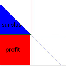
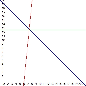
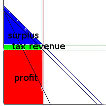
Land has an extremely high cost to create—for practical purposes, we can consider its supply fixed, that is, perfectly inelastic. If the market is competitive, so that landlords have no market power, then they will simply rent out all the land they have at whatever price the market will bear:

Inelastic_supply_competitive_labeled

This is like setting n = 0 and T = 0 in the above equations, the competitive ones.

Q = Q0

Q = Q_0 \\

P = PR – Q0/e

P = P_R – \frac{Q_0}{e} \\

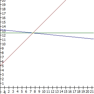
If we now introduce a tax, it will fall completely on the landlords, because they have little choice but to rent out all the land they have, and they can only rent it at a price—including tax—that the market will bear.

inelastic_supply_competitive_tax_labeled

Now we still have n = 0 but not T = 0.

Q = Q0

Q = Q_0 \\

P = PR – T – Q0/e

P = P_R – T – \frac{Q_0}{e} \\

The consumer surplus will be:

½ (Q)(PR – P – T) = 1/(2e)* Q02

\frac{1}{2}Q(P_R – P – T) = \frac{1}{2e}Q_0^2 \\

Notice how T isn’t in the result. The consumer surplus is unaffected by the tax.

The producer surplus, on the other hand, will be reduced by the tax:

(Q)(P) = (PR – T – Q0/e) Q0 = PR Q0 – 1/e Q02 – TQ0

(Q)(P) = (P_R – T – \frac{Q_0}{e})Q_0 = P_R Q_0 – \frac{1}{e} Q_0^2 – T Q_0 \\

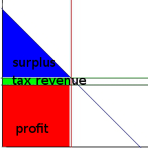
T appears linearly as TQ0, which is the same as the tax revenue. All the money goes directly from the landlord to the government, as we want if our goal is to redistribute wealth without raising rent.

But now suppose that the market is not competitive, and by tacit collusion or regulatory capture the landlords can exert some market power; this is quite likely the case in reality. Actually in reality we’re probably somewhere in between monopoly and competition, either oligopoly or monopolistic competitionwhich I will talk about a good deal more in a later post, I promise.

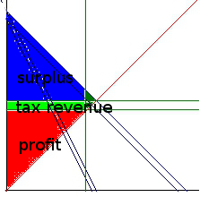
It could be that demand is still sufficiently high that even with their market power, landlords have an incentive to rent out all their available land, in which case the result will be the same as in the competitive market.

inelastic_supply_monopolistic_labeled

A tax will then fall completely on the landlords as before:

inelastic_supply_monopolistic_tax_labeled

Indeed, in this case it doesn’t really matter that the market is monopolistic; everything is the same as it would be under a competitive market. Notice how if you set n = 0, the monopolistic equations and the competitive equations come out exactly the same. The good news is, this is quite likely our actual situation! So even in the presence of significant market power the land tax can redistribute wealth in just the way we want.

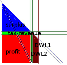
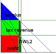
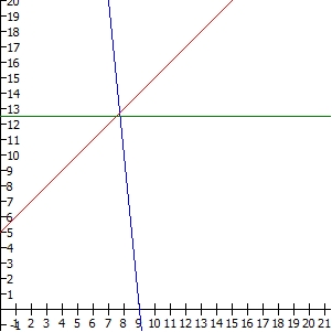
But there are a few other possibilities. One is that demand is not sufficiently high, so that the landlords’ market power causes them to actually hold back some land in order to raise the price:

zerobound_supply_monopolistic_labeled

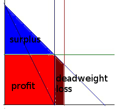
This will create some of what we call deadweight loss, in which some economic value is wasted. By restricting the land they rent out, the landlords make more profit, but the harm they cause to tenant is created than the profit they gain, so there is value wasted.

Now instead of setting n = 0, we actually set n = infinity. Why? Because the reason that the landlords restrict the land they sell is that their marginal revenue is actually negative beyond that point—they would actually get less money in total if they sold more land. Instead of being bounded by their cost of production (because they have none, the land is there whether they sell it or not), they are bounded by zero. (Once again we’ve hit upon a fundamental concept in economics, particularly macroeconomics, that I don’t have time to talk about today: the zero lower bound.) Thus, they can change quantity all they want (within a certain range) without changing the price, which is equivalent to a supply elasticity of infinity.

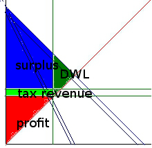
Introducing a tax will then exacerbate this deadweight loss (adding DWL2 to the original DWL1), because it provides even more incentive for the landlords to restrict the supply of land:

zerobound_supply_monopolistic_tax_labeled

Q = e/2*(PR – T)

Q = \frac{e}{2} \left(P_R – T\right)\\

P = 1/2*(PR – T)

P = \frac{1}{2} \left(P_R – T\right) \\

The quantity Q0 completely drops out, because it doesn’t matter how much land is available (as long as it’s enough); it only matters how much land it is profitable to rent out.

We can then find the consumer and producer surplus, and see that they are both reduced by the tax. The consumer surplus is as follows:

½ (Q)(PR – 1/2(PR – T)) = e/4*(PR2 – T2)

\frac{1}{2}Q \left( P_R – \frac{1}{2}left( P – T \right) \right) = \frac{e}{4}\left( P_R^2 – T^2 \right) \\

This time, the tax does have an effect on reducing the consumer surplus.

The producer surplus, on the other hand, will be:

(Q)(P) = 1/2*(PR – T)*e/2*(PR – T) = e/4*(PR – T)2

(Q)(P) = \frac{1}{2}\left(P_R – T \right) \frac{e}{2} \left(P_R – T\right) = \frac{e}{4} \left(P_R – T)^2 \\

Notice how it is also reduced by the tax—and no longer in a simple linear way.

The tax revenue is now a function of the demand:

TQ = e/2*T(PR – T)

T Q = \frac{e}{2} T (P_R – T) \\

If you add all these up, you’ll find that the sum is this:

e/2 * (PR^2 – T^2)

\frac{e}{2} \left(P_R^2 – T^2 \right) \\

The sum is actually reduced by an amount equal to e/2*T^2, which is the deadweight loss.

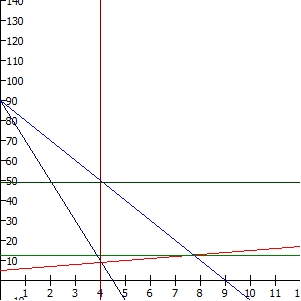
Finally there is an even worse scenario, in which the tax is so large that it actually creates an incentive to restrict land where none previously existed:

zerobound_supply_monopolistic_hugetax_labeled

Notice, however, that because the supply of land is inelastic the deadweight loss is still relatively small compared to the huge amount of tax revenue.

But actually this isn’t the whole story, because a land tax provides an incentive to get rid of land that you’re not profiting from. If this incentive is strong enough, the monopolistic power of landlords will disappear, as the unused land gets sold to more landholders or to the government. This is a way of avoiding the tax, but it’s one that actually benefits society, so we don’t mind incentivizing it.

Now, let’s compare this to our current system of property taxes, which include the value of buildings. Buildings are expensive to create, but we build them all the time; the supply of buildings is strongly dependent upon the price at which those buildings will sell. This makes for a supply curve that is somewhat elastic.

If the market were competitive and we had no taxes, it would be optimally efficient:

elastic_supply_competitive_labeled

Property taxes create an incentive to produce fewer buildings, and this creates deadweight loss. Notice that this happens even if the market is perfectly competitive:

elastic_supply_competitive_tax_labeled

Since both n and e are finite and nonzero, we’d need to use the whole equations: Since the algebra is such a mess, I don’t see any reason to subject you to it; but suffice it to say, the T does not drop out. Tenants do see their consumer surplus reduced, and the larger the tax the more this is so.

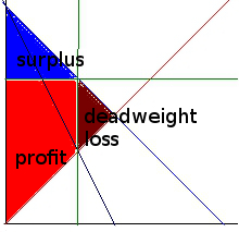
Now, suppose that the market for buildings is monopolistic, as it most likely is. This would create deadweight loss even in the absence of a tax:

elastic_supply_monopolistic_labeled

But a tax will add even more deadweight loss:

elastic_supply_monopolistic_tax_labeled

Once again, we’d need the full equations, and once again it’s a mess; but the result is, as before, that the tax gets passed on to the tenants in the form of more restricted sales and therefore higher rents.

Because of the finite supply elasticity, there’s no way that the tax can avoid raising the rent. As long as landlords have to pay more taxes when they build more or better buildings, they are going to raise the rent in those buildings accordingly—whether the market is competitive or not.

If the market is indeed monopolistic, there may be ways to bring the rent down: suppose we know what the competitive market price of rent should be, and we can establish rent control to that effect. If we are truly correct about the price to set, this rent control can not only reduce rent, it can actually reduce the deadweight loss:

effective_rent_control_tax_labeled

But if we set the rent control too low, or don’t properly account for the varying cost of different buildings, we can instead introduce a new kind of deadweight loss, by making it too expensive to make new buildings.

ineffective_rent_control_tax_labeled

In fact, what actually seems to happen is more complicated than that—because otherwise the number of buildings is obviously far too small, rent control is usually set to affect some buildings and not others. So what seems to happen is that the rent market fragments into two markets: One, which is too small, but very good for those few who get the chance to use it; and the other, which is unaffected by the rent control but is more monopolistic and therefore raises prices even further. This is why almost all economists are opposed to rent control (PDF); it doesn’t solve the problem of high rent and simply causes a whole new set of problems.

A land tax with a basic income, on the other hand, would help poor people at least as much as rent control presently does—probably a good deal more—without discouraging the production and maintenance of new apartment buildings.

But now we come to a key point: The land tax must be uniform per hectare.

If it is instead based on the value of the land, then this acts like a finite elasticity of supply; it provides an incentive to reduce the value of your own land in order to avoid the tax. As I showed above, this is particularly pernicious if the market is monopolistic, but even if it is competitive the effect is still there.

One exception I can see is if there are different tiers based on broad classes of land that it’s difficult to switch between, such as “land in Manhattan” versus “land in Brooklyn” or “desert land” versus “forest land”. But even this policy would have to be done very carefully, because any opportunity to substitute can create an opportunity to pass on the tax to someone else—for instance if land taxes are lower in Brooklyn developers are going to move to Brooklyn. Maybe we want that, in which case that is a good policy; but we should be aware of these sorts of additional consequences. The simplest way to avoid all these problems is to simply make the land tax uniform. And given the quantities we’re talking about—less than $3000 per hectare per year—it should be affordable for anyone except the very large landholders we’re trying to distribute wealth from in the first place.

The good news is, most economists would probably be on board with this proposal. After all, the neoclassical models themselves say it would be more efficient than our current system of rent control and property taxes—and the idea is at least as old as Adam Smith. Perhaps we can finally change the fact that the rent is too damn high.

What if you couldn’t own land?

JDN 2457145 EDT 20:49.

Today’s post we’re on the socialism scale somewhere near the The Guess Who, but not quite all the way to John Lennon. I’d like to questions one of the fundamental tenets of modern capitalism, but not the basic concept of private ownership itself:

What if you couldn’t own land?

Many things that you can own were more-or-less straightforwardly created by someone. A car, a computer, a television, a pair of shoes; for today let’s even take for granted intellectual property like books, movies, and songs; at least those things (“things”) were actually made by someone.

But land? We’re talking about chunks of the Earth here. They were here billions of years before us, and in all probability will be here billions of years after we’re gone. There’s no need to incentivize its creation; the vast majority of land was already here and did not need to be created. (I do have to say “the vast majority”, because in places like Japan, Hong Kong, and the Netherlands real estate has become so scarce that people do literally build land out into the sea. But this is something like 0.0001% of the world’s land.)

What we want to incentivize is land development; we want it to be profitable to build buildings and irrigate deserts, and yes, even cut down forests sometimes (though then there should be a carbon tax with credits for forested land to ensure that there isn’t too much incentive). Yet our current property tax system doesn’t do this very well; if you build bigger buildings, you end up paying more property taxes. Yes, you may also make some profit on the buildings—but it’s risky, and you may not get enough benefit to justify the added property taxes.

Moreover, we want to allocate land—we want some way of deciding who is allowed to use what land where and when (and perhaps why). Allowing land to be bought and sold is one way to do that, but it is not the only way.

Indeed, land ownership suffers from a couple of truly glaring flaws as an allocation system:

      1. It creates self-perpetuating inequality. Because land grows in value over time (due to population growth and urbanization, among other things), those who currently own land end up getting an ever-growing quantity of wealth while those who do not own land do not, and very likely end up having to pay ever-growing rents to the landlords. (I like calling them “landlords”; it really drives home the fact that our landholding system is still basically the same as it was under feudalism.) In fact, the recent rise in the share of income that goes to owners of capital rather than workers is almost entirely attributable to the rise in the price of real estate. As that post rightly recognizes, this does nothing to undermine Piketty’s central message of rising inequality due to capital income (pace The Washington Post); it merely tells us to focus on real estate instead of other forms of capital.
      2. It has no non-arbitrary allocation. If we want to decide who owns a car, we can ask questions like, “Who built it? Did someone buy it from them? Did they pay a fair price?”; if we want to decide who owns a book, we can ask questions like, “Who wrote it? Did they sell it to a publisher? What was the royalty rate?” That is, there is a clear original owner, and there is a sense of whether the transfer of ownership can be considered fair. But if we want to decide who owns a chunk of land, basically all we can ask is, “What does the deed say?” The owner is the owner because they are the owner; there’s no sense in which that ownership is fair. We certainly can’t go back to the original creation of the land, because that was due to natural forces gigayears ago. If we keep tracing the ownership backward, we will eventually end up with some guy (almost certainly a man, a White man in fact) with a gun who pointed that gun at other people and said, “This is mine.” This is true of basically all the land in the world (aside from those little bits of Japan and such); it was already there, and the only reason someone got to own it was because they said so and had a bigger gun. And a flag, perhaps: “Do you have a flag?” I suppose, in theory at least, there are a few ways of allocating land which seem less arbitrary: One would be to give everyone an equal amount. But this is practically very difficult: What do you do when the population changes? If you have 2% annual population growth, do you carve off 2% of everybody’s lot each year? Another would be to let people squat land, and automatically own the land that they live on—but again practical difficulties quickly become enormous. In any case, these two methods bear about as much resemblance to our actual allocation of land as a squirrel does to a Tyrannosaurus.

So, what else might we use? The system that makes the most sense to me is that we would own all land as a society. In practical terms this would mean that all land is Federal land, and if you want to use it for something, you need to pay rent to the government. There are many different ways the government could set the rent, but the most sensible might be to charge a flat rate per hectare regardless of where the land is or what it’s being used for, because that would maximize the incentive to develop the land. It would also make the rent fall entirely on the landowner, because the rent would be perfectly inelasticmeaning that you can’t change the quantity you make based on the price, because you aren’t making it; it’s just already sitting there.

Of course, this idea is obviously politically impossible in our current environment—or indeed any foreseeable political environment. I’m just fantasizing here, right?

Well, not quite. There is one thing we could do that would be economically quite similar to government-only land ownership; it’s called a land tax. The idea is incredibly simple: you just collect a flat tax per hectare of land. Economists have known that a land tax is efficient at providing revenue and reducing inequality since at least Adam Smith. So maybe ownership of land isn’t actually foundational to capitalism, after all; maybe we’ve just never fully gotten over feudalism. (I basically agree with Adam Smith, and for doing so I am often called a socialist.) The beautiful thing about a land tax is that it has a tax incidence in which the owners of the land end up bearing the full brunt of the tax.

Tax incidence is something it’s very important to understand; it would be on my list of the top ten economic principles that people should learn. We often have fierce political debates over who will actually write the check: Should employers pay the health insurance premium, or should employees? Will buyers pay sales tax, or sellers? Should we tax corporate profits or personal capital gains?

Please understand that I am not exaggerating when I say that these sorts of questions are totally irrelevant. It simply does not matter who actually writes the check; what matters is who bears the cost. Making the employer pay the health insurance premium doesn’t make the slightest difference if all they’re going to do is cut wages by the exact same amount. You can see the irrelevance of the fact that sellers pay sales tax every time you walk into a store—you always end up paying the price plus the tax, don’t you? (I found that the base price of most items was the same between Long Beach and Ann Arbor, but my total expenditure was always 3% more because of the 9% sales tax versus the 6%.) How do we determine who actually pays the tax? It depends on the elasticity—how easily can you change your behavior in order to avoid the tax? Can you find a different job because the health insurance premiums are too high? No? Then you’re probably paying that premium, even if your employer writes the check. If you can find a new job whenever you want, your employer might have to pay it for you even if you write the check.

The incidence of corporate taxes and taxes on capital gains are even more complicated, because it could affect the behavior of corporations in many different ways; indeed, many economists argue that the corporate tax simply results in higher unemployment or lower wages for workers. I don’t think that’s actually true, but I honestly can’t rule it out completely, precisely because corporate taxes are so complicated. You need to know all sorts of things about the structure of stock markets, and the freedom of trade, and the mobility of immigration… it’s a complete and total mess.

It’s because of tax incidence that a land tax makes so much sense; there’s no way for the landowner to escape it, other than giving up the land entirely. In particular, they can’t charge more for rent without being out-competed (unless landowners are really good at colluding—which might be true for large developers, but not individual landlords). Their elasticity is so low that they’re forced to bear the full cost of the tax.

If the land tax were high enough, it could eliminate the automatic growth in wealth that comes from holding land, and thereby reducing long-run inequality dramatically. The revenue could be used for my other favorite fiscal policy, the basic income—and real estate is a big enough part of our nation’s wealth that it’s actually entirely realistic to fund an $8,000 per person per year basic income entirely on land tax revenue. The total value of US land is about $14 trillion, and an $8,000 basic income for 320 million people would cost about $2.6 trillion; that’s only 19%. You’d actually want to make it a flat tax per hectare, so how much would that be? Well, 60% of US land is privately owned at present (no sense taxing the land the government already owns), and total US land area is about 9 million square kilometers, so to raise $2.5 trillion you’d need a tax of $289,000 per square kilometer, or $2,890 per hectare. If you own a hectare—which is bigger than most single-family lots—you’d only pay $2,890 per year in land tax, well within what most middle-class families could handle. But if you own 290,000 acres like Jeff Bezos, (that’s 117,000 hectares) you’re paying $338 million per year. Since Jeff Bezos has about $38 billion in net wealth, he can actually afford to pay that ($338 million per year is about one-tenth of what Jeff Bezos makes automatically on dividends), though he might consider selling off some of the land to avoid the taxes, which is exactly the sort of incentive we wanted to create.

Indeed, when I contemplate this policy I’m struck by the fact that it has basically no downside—usually in public policy you’re forced to make hard compromises and tradeoffs, but a land tax plus basic income is a system that carries almost no downsides at all. It won’t disincentivize investment, it won’t disincentivize working, it will dramatically reduce inequality, it will save the government a great deal of money on social welfare spending, and best of all it will eliminate poverty immediately and forever. The only people it would hurt at all are extremely rich, and they wouldn’t even be hurt very much, while it would benefit millions of people including some of the most needy.

Why aren’t we doing this already!?

Is marginal productivity fair?

JDN 2456963 PDT 11:11.

The standard economic equilibrium that is the goal of any neoclassical analysis is based on margins, rather than totals; what matters is not how much you have in all, but how much you get from each new one. This may be easier to understand with specific examples: The price of a product isn’t set by the total utility that you get from using that product; it’s set by the marginal utility that you get from each new unit. The wage of a worker isn’t set by their total value to the company; it’s set by the marginal value they provide with each additional hour of work. Formally, it’s not the value of the function f(x), it’s the derivative of the function, f'(x). (If you don’t know calculus, don’t worry about that last part; it isn’t that important to understand the basic concept.)

This is the standard modern explanation for Adam Smith’s “diamond-water paradox“: Why are diamonds so much more expensive than water, even though water is much more useful? Well, we have plenty of water, so the marginal utility of water isn’t very high; what are you really going to do with that extra liter? But we don’t have a lot of diamonds, so even though diamonds in general aren’t that useful, getting an extra diamond has a lot of benefit. (The units are a bit weird, as George Stigler once used to argue that Smith’s paradox is “meaningless”; but that’s silly. Let’s fix the units at “per kilogram”; a kilogram of diamonds is far, far more expensive than a kilogram of water.)

This explanation is obviously totally wrong, by the way; that’s not why diamonds are expensive. The marginal-utility argument makes sense for cars (or at least ordinary Fords and Toyotas, for reasons you’ll see in a minute), but it doesn’t explain diamonds. Diamonds are expensive for two reasons: First, the absolutely insane monopoly power of the De Beers cartel; as you might imagine, water would be really expensive too if it were also controlled by a single cartel with the power to fix prices and crush competitors. (For awhile De Beers executives had a standing warrant for their arrest in the United States; recently they pled guilty and paid fines—because, as we all know, rich people never go to prison.) And you can clearly see how diamond prices plummeted when the cartel was weakened in the 1980s. But Smith was writing long before DeBeers, and even now that De Beers only controls 40% of the market so we have an oligopoly instead of a monopoly (it’s a step in the right direction I guess), diamonds are still far more expensive than water. The real reason why diamonds are expensive is that diamonds are a Veblen good; you don’t buy diamonds because you actually want to use diamonds (maybe once in awhile, if you want to make a diamond saw or something). You buy diamonds in order to show off how rich you are. And if your goal is to show how rich you are, higher prices are good; you want it to be really expensive, you’re more likely to buy it if it’s really expensive. That’s why the marginal utility argument doesn’t work for Porsches and Ferraris; they’re Veblen goods too. If the price of a Ferrari suddenly dropped to $10,000, people would realize pretty quickly that they are hard to maintain, have very poor suspensions, and get awful gas mileage. It’s not like you can actually drive at 150 mph without getting some serious speeding tickets. (I guess they look nice?) But if the price of a Prius dropped to $10,000, everyone would buy one. For some people diamonds are also a speculation good; they hope to buy them at one price and sell them at a higher price. This is also how most trading in the stock market works, which is why I’m dubious of how well the stock market actually supports real investment. When we’re talking about Veblen goods and speculation goods, the sky is the limit; any price that someone can pay is a price they might sell at.

But all of that is a bit tangential. It’s worth thinking about all the ways that neoclassical theory doesn’t comport with reality, all the cases where price and marginal value become unhinged. But for today I’m going to give the neoclassicists the benefit of the doubt: Suppose it were true. Suppose that markets really were perfectly efficient and everything were priced at its marginal value. Would that even be a good thing?

I tend to focus most of my arguments on why a given part of our economic system deviates from optimal efficiency, because once you can convince economists of that they are immediately willing to try to fix it. But what if we had optimal efficiency? Most economists would say that we’re done, we’ve succeeded, everything is good now. (I am suddenly reminded of the Lego song, “Everything is Awesome.”) This notion is dangerously wrong.

A system could be perfectly efficient and still be horrifically unfair. This is particularly important when we’re talking about labor markets. A diamond or a bottle of water doesn’t have feelings; it doesn’t care what price you sell it at. More importantly it doesn’t have rights. People have feelings; people have rights. (And once again I’m back to Citizens United; a rat is more of a person than any corporation. We should stop calling them “rats” and “fat cats”, for this is an insult to the rodent and feline communities. No, only a human psychopath could ever be quite so corrupt.)

Of course when you sell a product, the person selling it cares how much you pay, but that will either trace back to someone’s labor—and labor markets are still the issue—or it won’t, in which case as far as I’m concerned it really doesn’t matter. If you make money simply by owning things, our society is giving you an enormous gift simply by allowing that capital income to exist; press the issue much more and we’d be well within our rights to confiscate every dime. Unless and until capital ownership is shared across the entire population and we can use it to create a post-scarcity society, capital income will be a necessary evil at best.

So let’s talk about labor markets. If you’ve taken any economics, you have probably seen a great many diagrams like this:

supply_demand2

The red line is labor supply, the blue line is labor demand. At the intersection is our glorious efficient market equilibrium, in this case at 7.5 hours of work per day (the x-axis) and $12.50 an hour (the y-axis). The green line is the wage, $12.50 per hour. But let’s stop and think for a moment about what this diagram really means.

What decides that red labor supply line? Do people just arbitrarily decide that they’re going to work 4 hours a day if they get paid $9 an hour, but 8 hours a day if they get paid $13 an hour? No, this line is meant to represent the marginal real cost of working. It’s the monetized value of your work effort and the opportunity cost of what else you could have been doing with your time. It rises because the more hours you work, the more stress it causes you and the more of your life it takes up. Working 4 hours a day, you probably had that time available anyway. Working 8 hours a day, you can fit it in. Working 12 hours a day, now you have no leisure at all. Working 16 hours a day, now you’re having trouble fitting in basic needs like food and sleep. Working 20 hours a day, you eat at work, you don’t get enough sleep, and you’re going to burn yourself out in no time. Why is it a straight line? Because we assume linear relationships to make the math easier. (No, really; that is literally the only reason. We call them “supply and demand curves” but almost always draw and calculate them as straight lines.)

Now let’s consider the blue labor demand line. Is this how much the “job creators” see fit to bestow upon you? No, it’s the marginal value of productivity. The first hour you work each day, you are focused and comfortable, and you can produce a lot of output. The second hour you’re just a little bit fatigued, so you can produce a bit less. By the time you get to hour 8, you’re exhausted, and producing noticeably less output. And if they pushed you past 16 hours, you’d barely produce anything at all. They multiply the amount of products you produce by the price at which they can sell those products, and that’s their demand for your labor. And once again we assume it’s a straight line just to make the math easier.

From this diagram you can calculate what is called employer surplus and worker surplus. Employer surplus is basically the same thing as profit. (It’s not exactly the same for some wonky technical reasons, but for our purposes they may as well be the same.) Worker surplus is a subtler concept; it’s the amount of money you receive minus the monetized value of your cost of working. So if that first hour of work was really easy and you were willing to do it for anything over $5, we take that $5 as your monetized cost of working (your “marginal willingness-to-accept“). Then if you are being paid $12.50 an hour, we infer that you must have gained $7.50 worth of utility from that exchange. (“$7.50 of utility” is a very weird concept, for reasons I’ll get into more in a later post; but it is actually the standard means of estimating utility in neoclassical economics. That’s one of the things I hope to change, actually.)

When you add these up for all the hours worked, the result becomes an integral, which is a formal mathematical way of saying “the area between those two lines”. In this case they are triangles of equal size, so we can just use the old standby A = 1/2*b*h. The area of each triangle is 1/2*7.5*7.5 = $28.13. From each day you work, you make $28.13 in consumer surplus and your employer makes $28.13 in profit.

And that seems fair, doesn’t it? You split it right down the middle. Both of you are better off than you were, and the economic benefits are shared equally. If this were really how labor markets work, that seems like how things ought to be.

But nothing in the laws of economics says that the two areas need to be equal. We tend to draw them that way out of an aesthetic desire for symmetry. But in general they are not, and in some cases they can be vastly unequal.

This happens if we have wildly different elasticities, which is a formal term for the relative rates of change of two things. An elasticity of labor supply of 1 would mean that for a 1% increase in wage you’re willing to work 1% more hours, while an elasticity of 10 would mean that for a 1% increase in wage you’re willing to work 10% more hours. Elasticities can also be negative; a labor demand elasticity of -1 would mean that for a 1% increase in wage your employer is willing to hire you for 1% fewer hours. In the graph above, the elasticity of labor supply is exactly 1. The elasticity of labor demand varies along the curve, but at the equilibrium it is about -1.6. The fact that the profits are shared equally is related to the fact that these two elasticities are close in magnitude but opposite in sign.

But now consider this equilibrium, in which I’ve raised the labor elasticity to 10. Notice that the wage and number of hours haven’t change; it’s still 7.5 hours at $12.50 per hour. But now the profits are shared quite unequally indeed; while the employer still gets $28.13, the value for the worker is only 1/2*7.5*0.75 = $2.81. In real terms this means we’ve switched from a job that starts off easy but quickly gets harder to a job that is hard to start with but never gets much harder than that.

elastic_supply

On the other hand what if the supply elasticity is only 0.1? Now the worker surplus isn’t even a triangle; it’s a trapezoid. The area of this trapezoid is 6*12.5+1/2*1.5*12.5 = $84.38. This job starts off easy and fun—so much so that you’d do it for free—but then after 6 hours a day it quickly becomes exhausting and you need to stop.

inelastic_supply

If we had to guess what these jobs are, my suggestion is that maybe the first one is a research assistant, the second one is a garbage collector, and the third one is a video game tester. And thus, even though they are paid about the same (I think that’s true in real life? They all make about $15 an hour or $30k a year), we all agree that the video game tester job is better than the research assistant job which is better than the garbage collector job—which is exactly what the worker surplus figures are saying.

What about the demand side? Here’s where it gets really unfair. Going back to our research assistant with a supply elasticity of 1, suppose they’re not really that good a researcher. Their output isn’t wrong, but it’s also not very interesting. They can do the basic statistics, but they aren’t very creative and they don’t have a deep intuition for the subject. This might produce a demand elasticity 10 times larger. The worker surplus remains the same, but the employer surplus is much lower. The triangle has an area 1/2*7.5*0.75 = $2.81.

elastic_demand

Now suppose that they are the best research assistant ever; let’s say we have a young Einstein. Everything he touches turns to gold, but even Einstein needs his beauty sleep (he actually did sleep about 10 hours a day, which is something I’ve always been delighted to have in common with him), so the total number of work hours still caps out at 7.5. It is entirely possible for the wage equilibrium to be exactly the same as it was for the lousy researcher, making the graph look like this:

inelastic_demand

You can’t even see the top of the triangle on this scale; it’s literally off the chart. The worker had a lower bound at zero, but there’s no comparable upper bound. (I suppose you could argue the lower bound shouldn’t be there either, since there are kinds of work you’d be willing to do even if you had to pay to do them—like, well, testing video games.) The top of the triangle is actually at about $90, as it turns out, so the area of employer surplus is 1/2*(90-12.5)*7.5 = $290.63. For every day he works, the company gets almost $300, but Einstein himself only gets $28.13 after you include what it costs him to work. (His gross pay is just wage*hours of course, so that’s $93.75.) The total surplus produced is $318.76. Einstein himself only gets a measly 8.9% of that.

So here we have three research assistants, who have very different levels of productivity, getting the same pay. But isn’t pay supposed to reflect productivity? Sort of; it’s supposed to reflect marginal productivity. Because Einstein gets worn out and produces at the same level as the mediocre researcher after 7.5 hours of work, since that’s where the equilibrium is that’s what they both get paid.

Now maybe Einstein should hold back; he could exercise some monopolistic power over his amazing brain. By only offering to work 4 hours a day, he can force the company to pay him at his marginal productivity for 4 hours a day, which turns out to be $49 an hour. Now he makes a gross pay of $196, with a worker surplus of $171.

monopoly_power

This diagram is a bit harder to read, so let me walk you through it. The light red and blue lines are the same as before. The darker blue line is the marginal revenue per hour for Einstein, once he factors in the fact that working more hours will mean accepting a lower wage. The optimum for him is when that marginal revenue curve crosses his marginal cost curve, which is the red supply curve. That decides how many hours he will work, namely 4. But that’s not the wage he gets; to find that, we move up vertically along the dark red line until we get the company’s demand curve. That tells us what wage the company is willing to pay for the level of marginal productivity Einstein has at 4 hours per day of work—which is the $49 wage he ends up making shown by the dark green line. The lighter lines show what happens if we have a competitive labor market, while the darker lines show what happens if Einstein exercises monopoly power.

The company still does pretty well on this deal; they now make an employer surplus of $82. Now, of the total $253 of economic surplus being made, Einstein takes 69%. It’s his brain, so him taking most of the benefit seems fair.

But you should notice something: This result is inefficient! There’s a whole triangle between 4 and 7.5 hours that nobody is getting; it’s called the deadweight loss. In this case it is $65.76, the difference between the total surplus in the efficient equilibrium and the inefficient equilibrium. In real terms, this means that research doesn’t get done because Einstein held back in order to demand a higher wage. That’s research that should be done—its benefit exceeds its cost—but nobody is doing it. Well now, maybe that doesn’t seem so fair after all. It seems selfish of him to not do research that needs done just so he can get paid more for what he does.

If Einstein has monopoly power, he gets a fair share but the market is inefficient. Removing Einstein’s monopoly power by some sort of regulation would bring us back to efficiency, but it would give most of his share to the company instead. Neither way seems right.

How do we solve this problem? I’m honestly not sure. First of all, we rarely know the actual supply and demand elasticities, and when we do it’s generally after painstaking statistical work to determine the aggregate elasticities, which aren’t even what we’re talking about here. These are individual workers.

Notice that the problem isn’t due to imperfect information; the company knows full well that Einstein is a golden goose, but they aren’t going to pay him any more than they have to.

We could just accept it, I suppose. As long as the productive work gets done, we could shrug our shoulders and not worry about the fact that corporations are capturing most of the value from the hard work of our engineers and scientists. That seems to be the default response, perhaps because it’s the easiest. But it sure doesn’t seem fair to me.

One solution might be for the company to voluntarily pay Einstein more, or offer him some sort of performance bonus. I wouldn’t rule out this possibility entirely, but this would require the company to be unusually magnanimous. This won’t happen at most corporations. It might happen for researchers at a university, where the administrators are fellow academics. Or it might happen to a corporate executive because other corporate executives feel solidarity for their fellow corporate executives.

That sort of solidarity is most likely why competition hasn’t driven down executive salaries. Theoretically shareholders would have an incentive to choose boards of directors who are willing to work for $20 an hour and elect CEOs who are willing to work for $30 an hour; but in practice old rich White guys feel solidarity with other old rich White guys, and even if there isn’t any direct quid pro quo there is still a general sense that because we are “the same kind of people” we should all look out for each other—and that’s how you get $50 million salaries. And then of course there’s the fact that even publicly-traded companies often have a handful of shareholders who control enough of the shares to win any vote.

In some industries, we don’t need to worry about this too much because productivity probably doesn’t really vary that much; just how good can a fry cook truly be? But this is definitely an issue for a lot of scientists and engineers, particularly at entry-level positions. Some scientists are an awful lot better than other scientists, but they still get paid the same.

Much more common however is the case where the costs of working vary. Some people may have few alternatives, so their opportunity cost is low, driving their wage down; but that doesn’t mean they actually deserve a lower wage. Or they may be disabled, making it harder to work long hours; but even though they work so much harder their pay is the same, so their net benefit is much smaller. Even though they aren’t any more productive, it still seems like they should be paid more to compensate them for that extra cost of working. At the other end are people who start in a position of wealth and power; they have a high opportunity cost because they have so many other options, so it may take very high pay to attract them; but why do they deserve to be paid more just because they have more to start with?

Another option would be some sort of redistribution plan, where we tax the people who are getting a larger share and give it to those who are getting a smaller share. The problem here arises in how exactly you arrange the tax. A theoretical “lump sum tax” where we just figure out the right amount of money and say “Person A: Give $217 to person B! No, we won’t tell you why!” would be optimally efficient because there’s no way it can distort markets if nobody sees it coming; but this is not something we can actually do in the real world. (It also seems a bit draconian; the government doesn’t even tax activities, they just demand arbitrary sums of money?) We’d have to tax profits, or sales, or income; and all of these could potentially introduce distortions and make the market less efficient.

We could offer some sort of publicly-funded performance bonus, and for scientists actually we do; it’s called the Nobel Prize. If you are truly the best of the best of the best as Einstein was, you may have a chance at winning the Nobel and getting $1.5 million. But of course that has to be funded somehow, and it only works for the very very top; it doesn’t make much difference to Jane Engineer who is 20% more productive than her colleagues.

I don’t find any of these solutions satisfying. This time I really can’t offer a good solution. But I think it’s important to keep the problem in mind. It’s important to always remember that “efficient” does not mean “fair”, and being paid at marginal productivity isn’t the same as being paid for overall productivity.