Tax incidence revisited, part 5: Who really pays the tax?

JDN 2457359

I think all the pieces are now in place to really talk about tax incidence.

In earlier posts I discussed how taxes have important downsides, then talked about how taxes can distort prices, then explained that taxes are actually what gives money its value. In the most recent post in the series, I used supply and demand curves to show precisely how taxes create deadweight loss.

Now at last I can get to the fundamental question: Who really pays the tax?

The common-sense answer would be that whoever writes the check to the government pays the tax, but this is almost completely wrong. It is right about one aspect, a sort of political economy notion, which is that if there is any trouble collecting the tax, it’s generally that person who is on the hook to pay it. But especially in First World countries, most taxes are collected successfully almost all the time. Tax avoidance—using loopholes to reduce your tax burden—is all over the place, but tax evasion—illegally refusing to pay the tax you owe—is quite rare. And for this political economy argument to hold, you really need significant amounts of tax evasion and enforcement against it.

The real economic answer is that the person who pays the tax is the person who bears the loss in surplus. In essence, the person who bears the tax is the person who is most unhappy about it.

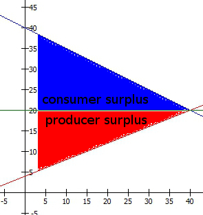
In the previous post in this series, I explained what surplus is, but it bears a brief repetition. Surplus is the value you get from purchases you make, in excess of the price you paid to get them. It’s measured in dollars, because that way we can read it right off the supply and demand curve. We should actually be adjusting for marginal utility of wealth and measuring in QALY, but that’s a lot harder so it rarely gets done.

In the graphs I drew in part 4, I already talked about how the deadweight loss is much greater if supply and demand are elastic than if they are inelastic. But in those graphs I intentionally set it up so that the elasticities of supply and demand were about the same. What if they aren’t?

Consider what happens if supply is very inelastic, but demand is very elastic. In fact, to keep it simple, lets suppose that supply is perfectly inelastic, but demand is perfectly elastic. This means that supply elasticity is 0, but demand elasticity is infinite.

The zero supply elasticity means that the worker would actually be willing to work up to their maximum hours for nothing, but is unwilling to go above that regardless of the wage. They have a specific amount of hours they want to work, regardless of what they are paid.

The infinite demand elasticity means that each hour of work is worth exactly the same amount the employer, with no diminishing returns. They have a specific wage they are willing to pay, regardless of how many hours it buys.

Both of these are quite extreme; it’s unlikely that in real life we would ever have an elasticity that is literally zero or infinity. But we do actually see elasticities that get very low or very high, and qualitatively they act the same way.

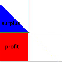
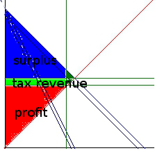
So let’s suppose as before that the wage is $20 and the number of hours worked is 40. The supply and demand graph actually looks a little weird: There is no consumer surplus whatsoever.

incidence_infinite_notax_surplus

Each hour is worth $20 to the employer, and that is what they shall pay. The whole graph is full of producer surplus; the worker would have been willing to work for free, but instead gets $20 per hour for 40 hours, so they gain a whopping $800 in surplus.

incidence_infinite_tax_surplus

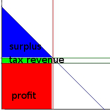
Now let’s implement a tax, say 50% to make it easy. (That’s actually a huge payroll tax, and if anybody ever suggested implementing that I’d be among the people pulling out a Laffer curve to show them why it’s a bad idea.)

Normally a tax would push the demand wage higher, but in this case $20 is exactly what they can afford, so they continue to pay exactly the same as if nothing had happened. This is the extreme example in which your “pre-tax” wage is actually your pre-tax wage, what you’d get if there hadn’t been a tax. This is the only such example—if demand elasticity is anything less than infinity, the wage you see listed as “pre-tax” will in fact be higher than what you’d have gotten in the absence of the tax.

The tax revenue is therefore borne entirely by the worker; they used to take home $20 per hour, but now they only get $10. Their new surplus is only $400, precisely 40% lower. The extra $400 goes directly to the government, which makes this example unusual in another way: There is no deadweight loss. The employer is completely unaffected; their surplus goes from zero to zero. No surplus is destroyed, only moved. Surplus is simply redistributed from the worker to the government, so the worker bears the entirety of the tax. Note that this is true regardless of who actually writes the check; I didn’t even have to include that in the model. Once we know that there was a tax imposed on each hour of work, the market prices decided who would bear the burden of that tax.

By Jove, we’ve actually found an example in which it’s fair to say “the government is taking my hard-earned money!” (I’m fairly certain if you replied to such people with “So you think your supply elasticity is zero but your employer’s demand elasticity is infinite?” you would be met with blank stares or worse.)

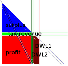
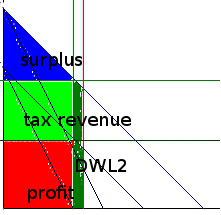
This is however quite an extreme case. Let’s try a more realistic example, where supply elasticity is very small, but not zero, and demand elasticity is very high, but not infinite. I’ve made the demand elasticity -10 and the supply elasticity 0.5 for this example.

incidence_supply_notax_surplus

Before the tax, the wage was $20 for 40 hours of work. The worker received a producer surplus of $700. The employer received a consumer surplus of only $80. The reason their demand is so elastic is that they are only barely getting more from each hour of work than they have to pay.

Total surplus is $780.

incidence_supply_tax_surplus

After the tax, the number of hours worked has dropped to 35. The “pre-tax” (demand) wage has only risen to $20.25. The after-tax (supply) wage the worker actually receives has dropped all the way to $10. The employer’s surplus has only fallen to $65.63, a decrease of $14.37 or 18%. Meanwhile the worker’s surplus has fallen all the way to $325, a decrease of $275 or 46%. The employer does feel the tax, but in both absolute and relative terms, the worker feels the tax much more than the employer does.

The tax revenue is $358.75, which means that the total surplus has been reduced to $749.38. There is now $30.62 of deadweight loss. Where both elasticities are finite and nonzero, deadweight loss is basically inevitable.

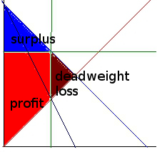
In this more realistic example, the burden was shared somewhat, but it still mostly fell on the worker, because the worker had a much lower elasticity. Let’s try turning the tables and making demand elasticity low while supply elasticity is high—in fact, once again let’s illustrate by using the extreme case of zero versus infinity.

In order to do this, I need to also set a maximum wage the employer is willing to pay. With nonzero elasticity, that maximum sort of came out automatically when the demand curve hits zero; but when elasticity is zero, the line is parallel so it never crosses. Let’s say in this case that the maximum is $50 per hour.

(Think about why we didn’t need to set a minimum wage for the worker when supply was perfectly inelastic—there already was a minimum, zero.)

incidence_infinite2_notax_surplus

This graph looks deceptively similar to the previous; basically all that has happened is the supply and demand curves have switched places, but that makes all the difference. Now instead of the worker getting all the surplus, it’s the employer who gets all the surplus. At their maximum wage of $50, they are getting $1200 in surplus.

Now let’s impose that same 50% tax again.

incidence_infinite2_tax_surplus

The worker will not accept any wage less than $20, so the demand wage must rise all the way to $40. The government will then receive $800 in revenue, while the employer will only get $400 in surplus. Notice again that the deadweight loss is zero. The employer will now bear the entire burden of the tax.

In this case the “pre-tax” wage is basically meaningless; regardless of the value of the tax the worker would receive the same amount, and the “pre-tax” wage is really just an accounting mechanism the government uses to say how large the tax is. They could just as well have said, “Hey employer, give us $800!” and the outcome would be the same. This is called a lump-sum tax, and they don’t work in the real world but are sometimes used for comparison. The thing about a lump-sum tax is that it doesn’t distort prices in any way, so in principle you could use it to redistribute wealth however you want. But in practice, there’s no way to implement a lump-sum tax that would be large enough to raise sufficient revenue but small enough to be affordable by the entire population. Also, a lump-sum tax is extremely regressive, hurting the poor tremendously while the rich feel nothing. (Actually the closest I can think of to a realistic lump-sum tax would be a basic income, which is essentially a negative lump-sum tax.)

I could keep going with more examples, but the basic argument is the same.

In general what you will find is that the person who bears a tax is the person who has the most to lose if less of that good is sold. This will mean their supply or demand is very inelastic and their surplus is very large.

Inversely, the person who doesn’t feel the tax is the person who has the least to lose if the good stops being sold. That will mean their supply or demand is very elastic and their surplus is very small.
Once again, it really does not matter how the tax is collected. It could be taken entirely from the employer, or entirely from the worker, or shared 50-50, or 60-40, or whatever. As long as it actually does get paid, the person who will actually feel the tax depends upon the structure of the market, not the method of tax collection. Raising “employer contributions” to payroll taxes won’t actually make workers take any more home; their “pre-tax” wages will simply be adjusted downward to compensate. Likewise, raising the “employee contribution” won’t actually put more money in the pockets of the corporation, it will just force them to raise wages to avoid losing employees. The actual amount that each party must contribute to the tax isn’t based on how the checks are written; it’s based on the elasticities of the supply and demand curves.

And that’s why I actually can’t get that strongly behind corporate taxes; even though they are formally collected from the corporation, they could simply be hurting customers or employees. We don’t actually know; we really don’t understand the incidence of corporate taxes. I’d much rather use income taxes or even sales taxes, because we understand the incidence of those.

Tax incidence revisited, part 4: Surplus and deadweight loss

JDN 2457355

I’ve already mentioned the fact that taxation creates deadweight loss, but in order to understand tax incidence it’s important to appreciate exactly how this works.

Deadweight loss is usually measured in terms of total economic surplus, which is a strange and deeply-flawed measure of value but relatively easy to calculate.

Surplus is based upon the concept of willingness-to-pay; the value of something is determined by the maximum amount of money you would be willing to pay for it.

This is bizarre for a number of reasons, and I think the most important one is that people differ in how much wealth they have, and therefore in their marginal utility of wealth. $1 is worth more to a starving child in Ghana than it is to me, and worth more to me than it is to a hedge fund manager, and worth more to a hedge fund manager than it is to Bill Gates. So when you try to set what something is worth based on how much someone will pay for it, which someone are you using?

People also vary, of course, in how much real value a good has to them: Some people like dark chocolate, some don’t. Some people love spicy foods and others despise them. Some people enjoy watching sports, others would rather read a book. A meal is worth a lot more to you if you haven’t eaten in days than if you just ate half an hour ago. That’s not actually a problem; part of the point of a market economy is to distribute goods to those who value them most. But willingness-to-pay is really the product of two different effects: The real effect, how much utility the good provides you; and the wealth effect, how your level of wealth affects how much you’d pay to get the same amount of utility. By itself, willingness-to-pay has no means of distinguishing these two effects, and actually I think one of the deepest problems with capitalism is that ultimately capitalism has no means of distinguishing these two effects. Products will be sold to the highest bidder, not the person who needs it the most—and that’s why Americans throw away enough food to end world hunger.

But for today, let’s set that aside. Let’s pretend that willingness-to-pay is really a good measure of value. One thing that is really nice about it is that you can read it right off the supply and demand curves.

When you buy something, your consumer surplus is the difference between your willingness-to-pay and how much you actually did pay. If a sandwich is worth $10 to you and you pay $5 to get it, you have received $5 of consumer surplus.

When you sell something, your producer surplus is the difference between how much you were paid and your willingness-to-accept, which is the minimum amount of money you would accept to part with it. If making that sandwich cost you $2 to buy ingredients and $1 worth of your time, your willingness-to-accept would be $3; if you then sell it for $5, you have received $2 of producer surplus.

Total economic surplus is simply the sum of consumer surplus and producer surplus. One of the goals of an efficient market is to maximize total economic surplus.

Let’s return to our previous example, where a 20% tax raised the original wage from $22.50 and thus resulted in an after-tax wage of $18.

Before the tax, the supply and demand curves looked like this:

equilibrium_notax

Consumer surplus is the area below the demand curve, above the price, up to the total number of goods sold. The basic reasoning behind this is that the demand curve gives the willingness-to-pay for each good, which decreases as more goods are sold because of diminishing marginal utility. So what this curve is saying is that the first hour of work was worth $40 to the employer, but each following hour was worth a bit less, until the 10th hour of work was only worth $35. Thus the first hour gave $40-$20 = $20 of surplus, while the 10th hour only gave $35-$20 = $15 of surplus.

Producer surplus is the area above the supply curve, below the price, again up to the total number of goods sold. The reasoning is the same: If the first hour of work cost $5 worth of time but the 10th hour cost $10 worth of time, the first hour provided $20-$5 = $15 in producer surplus, but the 10th hour only provided $20-$10 = $10 in producer surplus.

Imagine drawing a little 1-pixel-wide line straight down from the demand curve to the price for each hour and then adding up all those little lines into the total area under the curve, and similarly drawing little 1-pixel-wide lines straight up from the supply curve.

surplus

The employer was paying $20 * 40 = $800 for an amount of work that they actually valued at $1200 (the total area under the demand curve up to 40 hours), so they benefit by $400. The worker was being paid $800 for an amount of work that they would have been willing to accept $480 to do (the total area under the supply curve up to 40 hours), so they benefit $320. The sum of these is the total surplus $720.

equilibrium_notax_surplus

After the tax, the employer is paying $22.50 * 35 = $787.50, but for an amount of work that they only value at $1093.75, so their new surplus is only $306.25. The worker is receiving $18 * 35 = $630, for an amount of work they’d have been willing to accept $385 to do, so their new surplus is $245. Even when you add back in the government revenue of $4.50 * 35 = $157.50, the total surplus is still only $708.75. What happened to that extra $11.25 of value? It simply disappeared. It’s gone. That’s what we mean by “deadweight loss”. That’s why there is a downside to taxation.

equilibrium_tax_surplus

How large the deadweight loss is depends on the precise shape of the supply and demand curves, specifically on how elastic they are. Remember that elasticity is the proportional change in the quantity sold relative to the change in price. If increasing the price 1% makes you want to buy 2% less, you have a demand elasticity of -2. (Some would just say “2”, but then how do we say it if raising the price makes you want to buy more? The Law of Demand is more like what you’d call a guideline.) If increasing the price 1% makes you want to sell 0.5% more, you have a supply elasticity of 0.5.

If supply and demand are highly elastic, deadweight loss will be large, because even a small tax causes people to stop buying and selling a large amount of goods. If either supply or demand is inelastic, deadweight loss will be small, because people will more or less buy and sell as they always did regardless of the tax.

I’ve filled in the deadweight loss with brown in each of these graphs. They are designed to have the same tax rate, and the same price and quantity sold before the tax.

When supply and demand are elastic, the deadweight loss is large:

equilibrium_elastic_tax_surplus

But when supply and demand are inelastic, the deadweight loss is small:

equilibrium_inelastic_tax_surplus

Notice that despite the original price and the tax rate being the same, the tax revenue is also larger in the case of inelastic supply and demand. (The total surplus is also larger, but it’s generally thought that we don’t have much control over the real value and cost of goods, so we can’t generally make something more inelastic in order to increase total surplus.)

Thus, all other things equal, it is better to tax goods that are inelastic, because this will raise more tax revenue while producing less deadweight loss.

But that’s not all that elasticity does!

At last, the end of our journey approaches: In the next post in this series, I will explain how elasticity affects who actually ends up bearing the burden of the tax.

What you need to know about tax incidence

JDN 2457152 EDT 14:54.

I said in my previous post that I consider tax incidence to be one of the top ten things you should know about economics. If I actually try to make a top ten list, I think it goes something like this:

  1. Supply and demand
  2. Monopoly and oligopoly
  3. Externalities
  4. Tax incidence
  5. Utility, especially marginal utility of wealth
  6. Pareto-efficiency
  7. Risk and loss aversion
  8. Biases and heuristics, including sunk-cost fallacy, scope neglect, herd behavior, anchoring and representative heuristic
  9. Asymmetric information
  10. Winner-takes-all effect

So really tax incidence is in my top five things you should know about economics, and yet I still haven’t talked about it very much. Well, today I will. The basic principles of supply and demand I’m basically assuming you know, but I really should spend some more time on monopoly and externalities at some point.

Why is tax incidence so important? Because of one central fact: The person who pays the tax is not the person who writes the check.

It doesn’t matter whether a tax is paid by the buyer or the seller; it matters what the buyer and seller can do to avoid the tax. If you can change your behavior in order to avoid paying the tax—buy less stuff, or buy somewhere else, or deduct something—you will not bear the tax as much as someone else who can’t do anything to avoid the tax, even if you are the one who writes the check. If you can avoid it and they can’t, other parties in the transaction will adjust their prices in order to eat the tax on your behalf.

Thus, if you have a good that you absolutely must buy no matter what—like, say, table saltand then we make everyone who sells that good pay an extra $5 per kilogram, I can guarantee you that you will pay an extra $5 per kilogram, and the suppliers will make just as much money as they did before. (A salt tax would be an excellent way to redistribute wealth from ordinary people to corporations, if you’re into that sort of thing. Not that we have any trouble doing that in America.)

On the other hand, if you have a good that you’ll only buy at a very specific price—like, say, fast food—then we can make you write the check for a tax of an extra $5 per kilogram you use, and in real terms you’ll pay hardly any tax at all, because the sellers will either eat the cost themselves by lowering the prices or stop selling the product entirely. (A fast food tax might actually be a good idea as a public health measure, because it would reduce production and consumption of fast food—remember, heart disease is one of the leading causes of death in the United States, making cheeseburgers a good deal more dangerous than terrorists—but it’s a bad idea as a revenue measure, because rather than pay it, people are just going to buy and sell less.)

In the limit in which supply and demand are both completely fixed (perfectly inelastic), you can tax however you want and it’s just free redistribution of wealth however you like. In the limit in which supply and demand are both locked into a single price (perfectly elastic), you literally cannot tax that good—you’ll just eliminate production entirely. There aren’t a lot of perfectly elastic goods in the real world, but the closest I can think of is cash. If you instituted a 2% tax on all cash withdrawn, most people would stop using cash basically overnight. If you want a simple way to make all transactions digital, find a way to enforce a cash tax. When you have a perfect substitute available, taxation eliminates production entirely.

To really make sense out of tax incidence, I’m going to need a lot of a neoclassical economists’ favorite thing: Supply and demand curves. These things pop up everywhere in economics; and they’re quite useful. I’m not so sure about their application to things like aggregate demand and the business cycle, for example, but today I’m going to use them for the sort of microeconomic small-market stuff that they were originally designed for; and what I say here is going to be basically completely orthodox, right out of what you’d find in an ECON 301 textbook.

Let’s assume that things are linear, just to make the math easier. You’d get basically the same answers with nonlinear demand and supply functions, but it would be a lot more work. Likewise, I’m going to assume a unit tax on goods—like $2890 per hectare—as opposed to a proportional tax on sales—like 6% property tax—again, for mathematical simplicity.

The next concept I’m going to have to talk about is elasticitywhich is the proportional amount that quantity sold changes relative to price. If price increases 2% and you buy 4% less, you have a demand elasticity of -2. If price increases 2% and you buy 1% less, you have a demand elasticity of -1/2. If price increases 3% and you sell 6% more, you have a supply elasticity of 2. If price decreases 5% and you sell 1% less, you have a supply elasticity of 1/5.

Elasticity doesn’t have any units of measurement, it’s just a number—which is part of why we like to use it. It also has some very nice mathematical properties involving logarithms, but we won’t be needing those today.

The price that renters are willing and able to pay, the demand price PD will start at their maximum price, the reserve price PR, and then it will decrease linearly according to the quantity of land rented Q, according to a linear function (simply because we assumed that) which will vary according to a parameter e that represents the elasticity of demand (it isn’t strictly equal to it, but it’s sort of a linearization).

We’re interested in what is called the consumer surplus; it is equal to the total amount of value that buyers get from their purchases, converted into dollars, minus the amount they had to pay for those purchases. This we add to the producer surplus, which is the amount paid for those purchases minus the cost of producing themwhich is basically just the same thing as profit. Togerther the consumer surplus and producer surplus make the total economic surplus, which economists generally try to maximize. Because different people have different marginal utility of wealth, this is actually a really terrible idea for deep and fundamental reasons—taking a house from Mitt Romney and giving it to a homeless person would most definitely reduce economic surplus, even though it would obviously make the world a better place. Indeed, I think that many of the problems in the world, particularly those related to inequality, can be traced to the fact that markets maximize economic surplus rather than actual utility. But for now I’m going to ignore all that, and pretend that maximizing economic surplus is what we want to do.

You can read off the economic surplus straight from the supply and demand curves; it’s the area between the lines. (Mathematically, it’s an integral; but that’s equivalent to the area under a curve, and with straight lines they’re just triangles.) I’m going to call the consumer surplus just “surplus”, and producer surplus I’ll call “profit”.

Below the demand curve and above the price is the surplus, and below the price and above the supply curve is the profit:

elastic_supply_competitive_labeled

I’m going to be bold here and actually use equations! Hopefully this won’t turn off too many readers. I will give each equation in both a simple text format and in proper LaTeX. Remember, you can render LaTeX here.

PD = PR – 1/e * Q

P_D = P_R – \frac{1}{e} Q \\

The marginal cost that landlords have to pay, the supply price PS, is a bit weirder, as I’ll talk about more in a moment. For now let’s say that it is a linear function, starting at zero cost for some quantity Q0 and then increases linearly according to a parameter n that similarly represents the elasticity of supply.

PS = 1/n * (Q – Q0)

P_S = \frac{1}{n} \left( Q – Q_0 \right) \\

Now, if you introduce a tax, there will be a difference between the price that renters pay and the price that landlords receive—namely, the tax, which we’ll call T. I’m going to assume that, on paper, the landlord pays the whole tax. As I said above, this literally does not matter. I could assume that on paper the renter pays the whole tax, and the real effect on the distribution of wealth would be identical. All we’d have to do is set PD = P and PS = P – T; the consumer and producer surplus would end up exactly the same. Or we could do something in between, with P’D = P + rT and P’S = P – (1 – r) T.

Then, if the market is competitive, we just set the prices equal, taking the tax into account:

P = PD – T = PR – 1/e * Q – T = PS = 1/n * (Q – Q0)

P= P_D – T = P_R – \frac{1}{e} Q – T= P_S = \frac{1}{n} \left(Q – Q_0 \right) \\

P_R – 1/e * Q – T = 1/n * (Q – Q0)

P_R – \frac{1}{e} Q – T = \frac{1}{n} \left(Q – Q_0 \right) \\

Notice the equivalency here; if we set P’D = P + rT and P’S = P – (1 – r) T, so that the consumer now pays a fraction of the tax r.

P = P’D – rT = P_r – 1/e*Q = P’S + (1 – r) T + 1/n * (Q – Q0) + (1 – r) T

P^\prime_D – r T = P = P_R – \frac{1}{e} Q = P^\prime_S = \frac{1}{n} \left(Q – Q_0 \right) + (1 – r) T\\

The result is exactly the same:

P_R – 1/e * Q – T = 1/n * (Q – Q0)

P_R – \frac{1}{e} Q – T = \frac{1}{n} \left(Q – Q_0 \right) \\

I’ll spare you the algebra, but this comes out to:

Q = (PR – T)/(1/n + 1/e) + (Q0)/(1 + n/e)

Q = \frac{P_R – T}{\frac{1}{n} + \frac{1}{e}} + \frac{Q_0}{1 + \frac{n}{e}}

P = (PR – T)/(1+ n/e) – (Q0)/(e + n)

P = \frac{P_R – T}}{1 + \frac{n}{e}} – \frac{Q_0}{e+n} \\

That’s if the market is competitive.

If the market is a monopoly, instead of setting the prices equal, we set the price the landlord receives equal to the marginal revenue—which takes into account the fact that increasing the amount they sell forces them to reduce the price they charge everyone else. Thus, the marginal revenue drops faster than the price as the quantity sold increases.

After a bunch of algebra (and just a dash of calculus), that comes out to these very similar, but not quite identical, equations:

Q = (PR – T)/(1/n + 2/e) + (Q0)/(1+ 2n/e)

Q = \frac{P_R – T}{\frac{1}{n} + \frac{2}{e}} + \frac{Q_0}{1 + \frac{2n}{e}} \\

P = (PR – T)*((1/n + 1/e)/(1/n + 2/e) – (Q0)/(e + 2n)

P = \left( P_R – T\right)\frac{\frac{1}{n} + \frac{1}{e}}{\frac{1}{n} + \frac{2}{e}} – \frac{Q_0}{e+2n} \\

Yes, it changes some 1s into 2s. That by itself accounts for the full effect of monopoly. That’s why I think it’s worthwhile to use the equations; they are deeply elegant and express in a compact form all of the different cases. They look really intimidating right now, but for most of the cases we’ll consider these general equations simplify quite dramatically.

There are several cases to consider.

Land has an extremely high cost to create—for practical purposes, we can consider its supply fixed, that is, perfectly inelastic. If the market is competitive, so that landlords have no market power, then they will simply rent out all the land they have at whatever price the market will bear:

Inelastic_supply_competitive_labeled

This is like setting n = 0 and T = 0 in the above equations, the competitive ones.

Q = Q0

Q = Q_0 \\

P = PR – Q0/e

P = P_R – \frac{Q_0}{e} \\

If we now introduce a tax, it will fall completely on the landlords, because they have little choice but to rent out all the land they have, and they can only rent it at a price—including tax—that the market will bear.

inelastic_supply_competitive_tax_labeled

Now we still have n = 0 but not T = 0.

Q = Q0

Q = Q_0 \\

P = PR – T – Q0/e

P = P_R – T – \frac{Q_0}{e} \\

The consumer surplus will be:

½ (Q)(PR – P – T) = 1/(2e)* Q02

\frac{1}{2}Q(P_R – P – T) = \frac{1}{2e}Q_0^2 \\

Notice how T isn’t in the result. The consumer surplus is unaffected by the tax.

The producer surplus, on the other hand, will be reduced by the tax:

(Q)(P) = (PR – T – Q0/e) Q0 = PR Q0 – 1/e Q02 – TQ0

(Q)(P) = (P_R – T – \frac{Q_0}{e})Q_0 = P_R Q_0 – \frac{1}{e} Q_0^2 – T Q_0 \\

T appears linearly as TQ0, which is the same as the tax revenue. All the money goes directly from the landlord to the government, as we want if our goal is to redistribute wealth without raising rent.

But now suppose that the market is not competitive, and by tacit collusion or regulatory capture the landlords can exert some market power; this is quite likely the case in reality. Actually in reality we’re probably somewhere in between monopoly and competition, either oligopoly or monopolistic competitionwhich I will talk about a good deal more in a later post, I promise.

It could be that demand is still sufficiently high that even with their market power, landlords have an incentive to rent out all their available land, in which case the result will be the same as in the competitive market.

inelastic_supply_monopolistic_labeled

A tax will then fall completely on the landlords as before:

inelastic_supply_monopolistic_tax_labeled

Indeed, in this case it doesn’t really matter that the market is monopolistic; everything is the same as it would be under a competitive market. Notice how if you set n = 0, the monopolistic equations and the competitive equations come out exactly the same. The good news is, this is quite likely our actual situation! So even in the presence of significant market power the land tax can redistribute wealth in just the way we want.

But there are a few other possibilities. One is that demand is not sufficiently high, so that the landlords’ market power causes them to actually hold back some land in order to raise the price:

zerobound_supply_monopolistic_labeled

This will create some of what we call deadweight loss, in which some economic value is wasted. By restricting the land they rent out, the landlords make more profit, but the harm they cause to tenant is created than the profit they gain, so there is value wasted.

Now instead of setting n = 0, we actually set n = infinity. Why? Because the reason that the landlords restrict the land they sell is that their marginal revenue is actually negative beyond that point—they would actually get less money in total if they sold more land. Instead of being bounded by their cost of production (because they have none, the land is there whether they sell it or not), they are bounded by zero. (Once again we’ve hit upon a fundamental concept in economics, particularly macroeconomics, that I don’t have time to talk about today: the zero lower bound.) Thus, they can change quantity all they want (within a certain range) without changing the price, which is equivalent to a supply elasticity of infinity.

Introducing a tax will then exacerbate this deadweight loss (adding DWL2 to the original DWL1), because it provides even more incentive for the landlords to restrict the supply of land:

zerobound_supply_monopolistic_tax_labeled

Q = e/2*(PR – T)

Q = \frac{e}{2} \left(P_R – T\right)\\

P = 1/2*(PR – T)

P = \frac{1}{2} \left(P_R – T\right) \\

The quantity Q0 completely drops out, because it doesn’t matter how much land is available (as long as it’s enough); it only matters how much land it is profitable to rent out.

We can then find the consumer and producer surplus, and see that they are both reduced by the tax. The consumer surplus is as follows:

½ (Q)(PR – 1/2(PR – T)) = e/4*(PR2 – T2)

\frac{1}{2}Q \left( P_R – \frac{1}{2}left( P – T \right) \right) = \frac{e}{4}\left( P_R^2 – T^2 \right) \\

This time, the tax does have an effect on reducing the consumer surplus.

The producer surplus, on the other hand, will be:

(Q)(P) = 1/2*(PR – T)*e/2*(PR – T) = e/4*(PR – T)2

(Q)(P) = \frac{1}{2}\left(P_R – T \right) \frac{e}{2} \left(P_R – T\right) = \frac{e}{4} \left(P_R – T)^2 \\

Notice how it is also reduced by the tax—and no longer in a simple linear way.

The tax revenue is now a function of the demand:

TQ = e/2*T(PR – T)

T Q = \frac{e}{2} T (P_R – T) \\

If you add all these up, you’ll find that the sum is this:

e/2 * (PR^2 – T^2)

\frac{e}{2} \left(P_R^2 – T^2 \right) \\

The sum is actually reduced by an amount equal to e/2*T^2, which is the deadweight loss.

Finally there is an even worse scenario, in which the tax is so large that it actually creates an incentive to restrict land where none previously existed:

zerobound_supply_monopolistic_hugetax_labeled

Notice, however, that because the supply of land is inelastic the deadweight loss is still relatively small compared to the huge amount of tax revenue.

But actually this isn’t the whole story, because a land tax provides an incentive to get rid of land that you’re not profiting from. If this incentive is strong enough, the monopolistic power of landlords will disappear, as the unused land gets sold to more landholders or to the government. This is a way of avoiding the tax, but it’s one that actually benefits society, so we don’t mind incentivizing it.

Now, let’s compare this to our current system of property taxes, which include the value of buildings. Buildings are expensive to create, but we build them all the time; the supply of buildings is strongly dependent upon the price at which those buildings will sell. This makes for a supply curve that is somewhat elastic.

If the market were competitive and we had no taxes, it would be optimally efficient:

elastic_supply_competitive_labeled

Property taxes create an incentive to produce fewer buildings, and this creates deadweight loss. Notice that this happens even if the market is perfectly competitive:

elastic_supply_competitive_tax_labeled

Since both n and e are finite and nonzero, we’d need to use the whole equations: Since the algebra is such a mess, I don’t see any reason to subject you to it; but suffice it to say, the T does not drop out. Tenants do see their consumer surplus reduced, and the larger the tax the more this is so.

Now, suppose that the market for buildings is monopolistic, as it most likely is. This would create deadweight loss even in the absence of a tax:

elastic_supply_monopolistic_labeled

But a tax will add even more deadweight loss:

elastic_supply_monopolistic_tax_labeled

Once again, we’d need the full equations, and once again it’s a mess; but the result is, as before, that the tax gets passed on to the tenants in the form of more restricted sales and therefore higher rents.

Because of the finite supply elasticity, there’s no way that the tax can avoid raising the rent. As long as landlords have to pay more taxes when they build more or better buildings, they are going to raise the rent in those buildings accordingly—whether the market is competitive or not.

If the market is indeed monopolistic, there may be ways to bring the rent down: suppose we know what the competitive market price of rent should be, and we can establish rent control to that effect. If we are truly correct about the price to set, this rent control can not only reduce rent, it can actually reduce the deadweight loss:

effective_rent_control_tax_labeled

But if we set the rent control too low, or don’t properly account for the varying cost of different buildings, we can instead introduce a new kind of deadweight loss, by making it too expensive to make new buildings.

ineffective_rent_control_tax_labeled

In fact, what actually seems to happen is more complicated than that—because otherwise the number of buildings is obviously far too small, rent control is usually set to affect some buildings and not others. So what seems to happen is that the rent market fragments into two markets: One, which is too small, but very good for those few who get the chance to use it; and the other, which is unaffected by the rent control but is more monopolistic and therefore raises prices even further. This is why almost all economists are opposed to rent control (PDF); it doesn’t solve the problem of high rent and simply causes a whole new set of problems.

A land tax with a basic income, on the other hand, would help poor people at least as much as rent control presently does—probably a good deal more—without discouraging the production and maintenance of new apartment buildings.

But now we come to a key point: The land tax must be uniform per hectare.

If it is instead based on the value of the land, then this acts like a finite elasticity of supply; it provides an incentive to reduce the value of your own land in order to avoid the tax. As I showed above, this is particularly pernicious if the market is monopolistic, but even if it is competitive the effect is still there.

One exception I can see is if there are different tiers based on broad classes of land that it’s difficult to switch between, such as “land in Manhattan” versus “land in Brooklyn” or “desert land” versus “forest land”. But even this policy would have to be done very carefully, because any opportunity to substitute can create an opportunity to pass on the tax to someone else—for instance if land taxes are lower in Brooklyn developers are going to move to Brooklyn. Maybe we want that, in which case that is a good policy; but we should be aware of these sorts of additional consequences. The simplest way to avoid all these problems is to simply make the land tax uniform. And given the quantities we’re talking about—less than $3000 per hectare per year—it should be affordable for anyone except the very large landholders we’re trying to distribute wealth from in the first place.

The good news is, most economists would probably be on board with this proposal. After all, the neoclassical models themselves say it would be more efficient than our current system of rent control and property taxes—and the idea is at least as old as Adam Smith. Perhaps we can finally change the fact that the rent is too damn high.