Do we always want to internalize externalities?

2016-02-172016-02-17 pnrj core principles, critique of neoclassical economics, public policy cake, consumer surplus, deadweight loss, externalities, inequality, Jonas Salk, marginal utility, Nobel Prize, QALY, surplus, technology, utility, wealth

JDN 2457437

I often talk about the importance of externalities—a full discussion in this earlier post, and one of their important implications, the tragedy of the commons, in another. Briefly, externalities are consequences of actions incurred upon people who did not perform those actions. Anything I do affecting you that you had no say in, is an externality.

Usually I’m talking about how we want to internalize externalities, meaning that we set up a system of incentives to make it so that the consequences fall upon the people who chose the actions instead of anyone else. If you pollute a river, you should have to pay to clean it up. If you assault someone, you should serve jail time as punishment. If you invent a new technology, you should be rewarded for it. These are all attempts to internalize externalities.

But today I’m going to push back a little, and ask whether we really always want to internalize externalities. If you think carefully, it’s not hard to come up with scenarios where it actually seems fairer to leave the externality in place, or perhaps reduce it somewhat without eliminating it.

For example, suppose indeed that someone invents a great new technology. To be specific, let’s think about Jonas Salk, inventing the polio vaccine. This vaccine saved the lives of thousands of people and saved millions more from pain and suffering. Its value to society is enormous, and of course Salk deserved to be rewarded for it.

But we did not actually fully internalize the externality. If we had, every family whose child was saved from polio would have had to pay Jonas Salk an amount equal to what they saved on medical treatments as a result, or even an amount somehow equal to the value of their child’s life (imagine how offended people would get if you asked that on a survey!). Those millions of people spared from suffering would need to each pay, at minimum, thousands of dollars to Jonas Salk, making him of course a billionaire.

And indeed this is more or less what would have happened, if he had been willing and able to enforce a patent on the vaccine. The inability of some to pay for the vaccine at its monopoly prices would add some deadweight loss, but even that could be removed if Salk Industries had found a way to offer targeted price vouchers that let them precisely price-discriminate so that every single customer paid exactly what they could afford to pay. If that had happened, we would have fully internalized the externality and therefore maximized economic efficiency.

But doesn’t that sound awful? Doesn’t it sound much worse than what we actually did, where Jonas Salk received a great deal of funding and support from governments and universities, and lived out his life comfortably upper-middle class as a tenured university professor?

Now, perhaps he should have been awarded a Nobel Prize—I take that back, there’s no “perhaps” about it, he definitely should have been awarded a Nobel Prize in Medicine, it’s absurd that he did not—which means that I at least do feel the externality should have been internalized a bit more than it was. But a Nobel Prize is only 10 million SEK, about $1.1 million. That’s about enough to be independently wealthy and live comfortably for the rest of your life; but it’s a small fraction of the roughly $7 billion he could have gotten if he had patented the vaccine. Yet while the possible world in which he wins a Nobel is better than this one, I’m fairly well convinced that the possible world in which he patents the vaccine and becomes a billionaire is considerably worse.

Internalizing externalities makes sense if your goal is to maximize total surplus (a concept I explain further in the linked post), but total surplus is actually a terrible measure of human welfare.

Total surplus counts every dollar of willingness-to-pay exactly the same across different people, regardless of whether they live on $400 per year or $4 billion.

It also takes no account whatsoever of how wealth is distributed. Suppose a new technology adds $10 billion in wealth to the world. As far as total surplus, it makes no difference whether that $10 billion is spread evenly across the entire planet, distributed among a city of a million people, concentrated in a small town of 2,000, or even held entirely in the bank account of a single man.

Particularly a propos of the Salk example, total surplus makes no distinction between these two scenarios: a perfectly-competitive market where everything is sold at a fair price, and a perfectly price-discriminating monopoly, where everything is sold at the very highest possible price each person would be willing to pay.

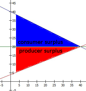
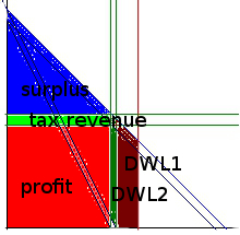
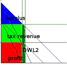
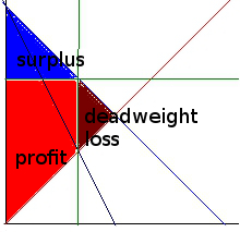
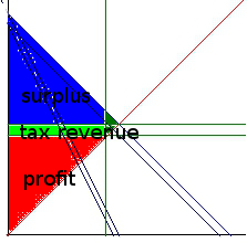
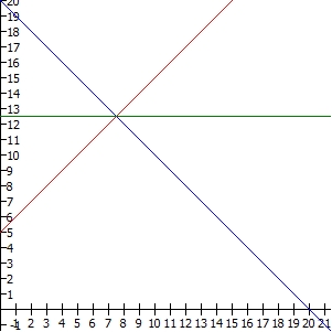
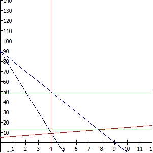
This is a perfectly-competitive market, where the benefits are more or less equally (in this case exactly equally, but that need not be true in real life) between sellers and buyers:

elastic_supply_competitive_labeled

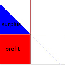
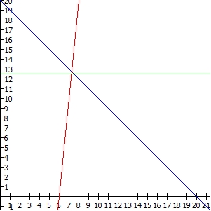
This is a perfectly price-discriminating monopoly, where the benefits accrue entirely to the corporation selling the good:

elastic_supply_price_discrimination

In the former case, the company profits, consumers are better off, everyone is happy. In the latter case, the company reaps all the benefits and everyone else is left exactly as they were. In real terms those are obviously very different outcomes—the former being what we want, the latter being the cyberpunk dystopia we seem to be hurtling mercilessly toward. But in terms of total surplus, and therefore the kind of “efficiency” that is maximize by internalizing all externalities, they are indistinguishable.

In fact (as I hope to publish a paper about at some point), the way willingness-to-pay works, it weights rich people more. Redistributing goods from the poor to the rich will typically increase total surplus.

Here’s an example. Suppose there is a cake, which is sufficiently delicious that it offers 2 milliQALY in utility to whoever consumes it (this is a truly fabulous cake). Suppose there are two people to whom we might give this cake: Richie, who has $10 million in annual income, and Hungry, who has only $1,000 in annual income. How much will each of them be willing to pay?

Well, assuming logarithmic marginal utility of wealth (which is itself probably biasing slightly in favor of the rich), 1 milliQALY is about $1 to Hungry, so Hungry will be willing to pay $2 for the cake. To Richie, however, 1 milliQALY is about $10,000; so he will be willing to pay a whopping $20,000 for this cake.

What this means is that the cake will almost certainly be sold to Richie; and if we proposed a policy to redistribute the cake from Richie to Hungry, economists would emerge to tell us that we have just reduced total surplus by $19,998 and thereby committed a great sin against economic efficiency. They will cajole us into returning the cake to Richie and thus raising total surplus by $19,998 once more.

This despite the fact that I stipulated that the cake is worth just as much in real terms to Hungry as it is to Richie; the difference is due to their wildly differing marginal utility of wealth.

Indeed, it gets worse, because even if we suppose that the cake is worth much more in real utility to Hungry—because he is in fact hungry—it can still easily turn out that Richie’s willingness-to-pay is substantially higher. Suppose that Hungry actually gets 20 milliQALY out of eating the cake, while Richie still only gets 2 milliQALY. Hungry’s willingness-to-pay is now $20, but Richie is still going to end up with the cake.

Now, if your thought is, “Why would Richie pay $20,000, when he can go to another store and get another cake that’s just as good for $20?” Well, he wouldn’t—but in the sense we mean for total surplus, willingness-to-pay isn’t just what you’d actually be willing to pay given the actual prices of the goods, but the absolute maximum price you’d be willing to pay to get that good under any circumstances. It is instead the marginal utility of the good divided by your marginal utility of wealth. In this sense the cake is “worth” $20,000 to Richie, and “worth” substantially less to Hungry—but not because it’s actually worth less in real terms, but simply because Richie has so much more money.

Even economists often equate these two, implicitly assuming that we are spending our money up to the point where our marginal willingness-to-pay is the actual price we choose to pay; but in general our willingness-to-pay is higher than the price if we are willing to buy the good at all. The consumer surplus we get from goods is in fact equal to the difference between willingness-to-pay and actual price paid, summed up over all the goods we have purchased.

Internalizing all externalities would definitely maximize total surplus—but would it actually maximize happiness? Probably not.

If you asked most people what their marginal utility of wealth is, they’d have no idea what you’re talking about. But most people do actually have an intuitive sense that a dollar is worth more to a homeless person than it is to a millionaire, and that’s really all we mean by diminishing marginal utility of wealth.

I think the reason we’re uncomfortable with the idea of Jonas Salk getting $7 billion from selling the polio vaccine, rather than the same number of people getting the polio vaccine and Jonas Salk only getting the $1.1 million from a Nobel Prize, is that we intuitively grasp that after that $1.1 million makes him independently wealthy, the rest of the money is just going to sit in some stock account and continue making even more money, while if we’d let the families keep it they would have put it to much better use raising their children who are now protected from polio. We do want to reward Salk for his great accomplishment, but we don’t see why we should keep throwing cash at him when it could obviously be spent in better ways.

And indeed I think this intuition is correct; great accomplishments—which is to say, large positive externalities—should be rewarded, but not in direct proportion. Maybe there should be some threshold above which we say, “You know what? You’re rich enough now; we can stop giving you money.” Or maybe it should simply damp down very quickly, so that a contribution which is worth $10 billion to the world pays only slightly more than one that is worth $100 million, but a contribution that is worth $100,000 pays considerably more than one which is only worth $10,000.

What it ultimately comes down to is that if we make all the benefits incur to the person who did it, there aren’t any benefits anymore. The whole point of Jonas Salk inventing the polio vaccine (or Einstein discovering relativity, or Darwin figuring out natural selection, or any great achievement) is that it will benefit the rest of humanity, preferably on to future generations. If you managed to fully internalize that externality, this would no longer be true; Salk and Einstein and Darwin would have become fabulously wealthy, and then somehow we’d all have to continue paying into their estates or something an amount equal to the benefits we received from their discoveries. (Every time you use your GPS, pay a royalty to the Einsteins. Every time you take a pill, pay a royalty to the Darwins.) At some point we’d probably get fed up and decide we’re no better off with them than without them—which is exactly by construction how we should feel if the externality were fully internalized.

Internalizing negative externalities is much less problematic—it’s your mess, clean it up. We don’t want other people to be harmed by your actions, and if we can pull that off that’s fantastic. (In reality, we usually can’t fully internalize negative externalities, but we can at least try.)

But maybe internalizing positive externalities really isn’t so great after all.

Tax incidence revisited, part 4: Surplus and deadweight loss

2015-11-282015-12-01 pnrj core principles, critique of neoclassical economics, public policy consumer surplus, deadweight loss, economic surplus, elasticity, producer surplus, supply and demand, surplus, taxation, taxes, willingness-to-accept, willingness-to-pay

JDN 2457355

I’ve already mentioned the fact that taxation creates deadweight loss, but in order to understand tax incidence it’s important to appreciate exactly how this works.

Deadweight loss is usually measured in terms of total economic surplus, which is a strange and deeply-flawed measure of value but relatively easy to calculate.

Surplus is based upon the concept of willingness-to-pay; the value of something is determined by the maximum amount of money you would be willing to pay for it.

This is bizarre for a number of reasons, and I think the most important one is that people differ in how much wealth they have, and therefore in their marginal utility of wealth. $1 is worth more to a starving child in Ghana than it is to me, and worth more to me than it is to a hedge fund manager, and worth more to a hedge fund manager than it is to Bill Gates. So when you try to set what something is worth based on how much someone will pay for it, which someone are you using?

People also vary, of course, in how much real value a good has to them: Some people like dark chocolate, some don’t. Some people love spicy foods and others despise them. Some people enjoy watching sports, others would rather read a book. A meal is worth a lot more to you if you haven’t eaten in days than if you just ate half an hour ago. That’s not actually a problem; part of the point of a market economy is to distribute goods to those who value them most. But willingness-to-pay is really the product of two different effects: The real effect, how much utility the good provides you; and the wealth effect, how your level of wealth affects how much you’d pay to get the same amount of utility. By itself, willingness-to-pay has no means of distinguishing these two effects, and actually I think one of the deepest problems with capitalism is that ultimately capitalism has no means of distinguishing these two effects. Products will be sold to the highest bidder, not the person who needs it the most—and that’s why Americans throw away enough food to end world hunger.

But for today, let’s set that aside. Let’s pretend that willingness-to-pay is really a good measure of value. One thing that is really nice about it is that you can read it right off the supply and demand curves.

When you buy something, your consumer surplus is the difference between your willingness-to-pay and how much you actually did pay. If a sandwich is worth $10 to you and you pay $5 to get it, you have received $5 of consumer surplus.

When you sell something, your producer surplus is the difference between how much you were paid and your willingness-to-accept, which is the minimum amount of money you would accept to part with it. If making that sandwich cost you $2 to buy ingredients and $1 worth of your time, your willingness-to-accept would be $3; if you then sell it for $5, you have received $2 of producer surplus.

Total economic surplus is simply the sum of consumer surplus and producer surplus. One of the goals of an efficient market is to maximize total economic surplus.

Let’s return to our previous example, where a 20% tax raised the original wage from $22.50 and thus resulted in an after-tax wage of $18.

Before the tax, the supply and demand curves looked like this:

equilibrium_notax

Consumer surplus is the area below the demand curve, above the price, up to the total number of goods sold. The basic reasoning behind this is that the demand curve gives the willingness-to-pay for each good, which decreases as more goods are sold because of diminishing marginal utility. So what this curve is saying is that the first hour of work was worth $40 to the employer, but each following hour was worth a bit less, until the 10^th hour of work was only worth $35. Thus the first hour gave $40-$20 = $20 of surplus, while the 10^th hour only gave $35-$20 = $15 of surplus.

Producer surplus is the area above the supply curve, below the price, again up to the total number of goods sold. The reasoning is the same: If the first hour of work cost $5 worth of time but the 10^th hour cost $10 worth of time, the first hour provided $20-$5 = $15 in producer surplus, but the 10^th hour only provided $20-$10 = $10 in producer surplus.

Imagine drawing a little 1-pixel-wide line straight down from the demand curve to the price for each hour and then adding up all those little lines into the total area under the curve, and similarly drawing little 1-pixel-wide lines straight up from the supply curve.

surplus

The employer was paying $20 * 40 = $800 for an amount of work that they actually valued at $1200 (the total area under the demand curve up to 40 hours), so they benefit by $400. The worker was being paid $800 for an amount of work that they would have been willing to accept $480 to do (the total area under the supply curve up to 40 hours), so they benefit $320. The sum of these is the total surplus $720.

equilibrium_notax_surplus

After the tax, the employer is paying $22.50 * 35 = $787.50, but for an amount of work that they only value at $1093.75, so their new surplus is only $306.25. The worker is receiving $18 * 35 = $630, for an amount of work they’d have been willing to accept $385 to do, so their new surplus is $245. Even when you add back in the government revenue of $4.50 * 35 = $157.50, the total surplus is still only $708.75. What happened to that extra $11.25 of value? It simply disappeared. It’s gone. That’s what we mean by “deadweight loss”. That’s why there is a downside to taxation.

equilibrium_tax_surplus

How large the deadweight loss is depends on the precise shape of the supply and demand curves, specifically on how elastic they are. Remember that elasticity is the proportional change in the quantity sold relative to the change in price. If increasing the price 1% makes you want to buy 2% less, you have a demand elasticity of -2. (Some would just say “2”, but then how do we say it if raising the price makes you want to buy more? The Law of Demand is more like what you’d call a guideline.) If increasing the price 1% makes you want to sell 0.5% more, you have a supply elasticity of 0.5.

If supply and demand are highly elastic, deadweight loss will be large, because even a small tax causes people to stop buying and selling a large amount of goods. If either supply or demand is inelastic, deadweight loss will be small, because people will more or less buy and sell as they always did regardless of the tax.

I’ve filled in the deadweight loss with brown in each of these graphs. They are designed to have the same tax rate, and the same price and quantity sold before the tax.

When supply and demand are elastic, the deadweight loss is large:

equilibrium_elastic_tax_surplus

But when supply and demand are inelastic, the deadweight loss is small:

equilibrium_inelastic_tax_surplus

Notice that despite the original price and the tax rate being the same, the tax revenue is also larger in the case of inelastic supply and demand. (The total surplus is also larger, but it’s generally thought that we don’t have much control over the real value and cost of goods, so we can’t generally make something more inelastic in order to increase total surplus.)

Thus, all other things equal, it is better to tax goods that are inelastic, because this will raise more tax revenue while producing less deadweight loss.

But that’s not all that elasticity does!

At last, the end of our journey approaches: In the next post in this series, I will explain how elasticity affects who actually ends up bearing the burden of the tax.

Tax Incidence Revisited, Part 1: The downside of taxes

2015-11-082015-11-08 pnrj core principles, public policy alcohol, alcohol tax, crime, deadweight loss, Denmark, externalities, Jeb!, Laffer Curve, land tax, lead, Marco Rubio, Pigovian tax, Reaganomics, supply-side, tax incidence, taxation, taxes, trickle-down, voodoo economics

JDN 2457345 EST 22:02

As I was writing this, it was very early (I had to wake up at 04:30) and I was groggy, because we were on an urgent road trip to Pennsylvania for the funeral of my aunt who died quite suddenly a few days ago. I have since edited this post more thoroughly to minimize the impact of my sleep deprivation upon its content. Actually maybe this is a good thing; the saying goes, “write drunk, edit sober” and sleep deprivation and alcohol have remarkably similar symptoms, probably because alcohol is GABA-ergic and GABA is involved in sleep regulation.

Awhile ago I wrote a long post on tax incidence, but the primary response I got was basically the online equivalent of a perplexed blank stare. Struck once again by the Curse of Knowledge, I underestimated the amount of background knowledge necessary to understand my explanation. But tax incidence is very important for public policy, so I really would like to explain it.

Therefore I am now starting again, slower, in smaller pieces. Today’s piece is about the downsides of taxation in general, why we don’t just raise taxes as high as we feel like and make the government roll in dough.

To some extent this is obvious; if income tax were 100%, why would anyone bother working for a salary? You might still work for fulfillment, or out of a sense of duty, or simply because you enjoy what you do—after all, most artists and musicians are hardly in it for the money. But many jobs are miserable and not particularly fulfilling, yet still need to get done. How many janitors or bus drivers work purely for the sense of fulfillment it gives them? Mostly they do it to pay the bills—and if income tax were 100%, it wouldn’t anymore. The formal economy would basically collapse, and then nobody would end up actually paying that 100% tax—so the government would actually get very little revenue, if any.

At the other end of the scale, it’s kind of obvious that if your taxes are all 0% you don’t get any revenue. This is actually more feasible than it may sound; provided you spend only a very small amount (say, 4% of GDP, though that’s less than any country actually spends—maybe you could do 6% like Bangladesh) and you can still get people to accept your currency, you could, in principle, have a government that funds its spending entirely by means of printing money, and could do this indefinitely. In practice, that has never been done, and the really challenging part is getting people to accept your money if you don’t collect taxes in it. One of the more counter-intuitive aspects of modern monetary theory (or perhaps I should capitalize it, Modern Monetary Theory, though the part I agree with is not that different from standard Keynesian theory) is that taxation is the primary mechanism by which money acquires its value.

And then of course with intermediate tax rates such as 20%, 30%, and 50% that actual countries actually use, we do get some positive amount of revenue.

Everything I’ve said so far may seem pretty obvious. Yeah, usually taxes raise revenue, but if you taxed at 0% or 100% they wouldn’t; so what?

Well, this leads to quite an important result. Assuming that tax revenue is continuous (which isn’t quite true, but since we can collect taxes in fractions of a percent and pay in pennies, it’s pretty close), it follows directly from the Extreme Value Theorem that there is in fact a revenue-maximizing tax rate. Both below and above that tax rate, the government takes in less total money. These theorems don’t tell us what the revenue-maximizing rate is; but they tell us that it must exist, somewhere between 0% and 100%.

Indeed, it follows that there is what we call the Laffer Curve, a graph of tax revenue as a function of tax rate, and it is in fact a curve, as opposed to the straight line it would be if taxes had no effect on the rest of the economy.

Very roughly, it looks something like this (the blue curve is my sketch of the real-world Laffer curve, while the red line is what it would be if taxes had no distortionary effects):

Now, the Laffer curve has been abused many times; in particular, it’s been used to feed into the “trickle-down” “supply-side” Reaganomics that has been rightly derided as “voodoo economics” by serious economists. Jeb Bush (or should I say, Jeb!) and Marco Rubio would have you believe that we are on the right edge of the Laffer curve, and we could actually increase tax revenue by cutting taxes, particularly on capital gains and incomes at the top 1%; that’s obviously false. We tried that, it didn’t work. Even theoretically we probably should have known that it wouldn’t; but now that we’ve actually done the experiment and it failed, there should be no serious doubt anymore.

No, we are on the left side of the Laffer curve, where increasing taxes increases revenue, much as you’d intuitively expect. It doesn’t quite increase one-to-one, because adding more taxes does make the economy less efficient; but from where we currently stand, a 1% increase in taxes leads to about a 0.9% increase in revenue (actually estimated as between 0.78% and 0.99%).

Denmark may be on the right side of the Laffer curve, where they could raise more revenue by decreasing tax rates (even then I’m not so sure). But Denmark’s tax rates are considerably higher than ours; while in the US we pay about 2 7% of GDP in taxes, folks in Denmark pay 49% of GDP in taxes.

The fact remains, however, that there is a Laffer curve, and no serious economist would dispute this. Increasing taxes does in fact create distortions in the economy, and as a result raising tax rates does not increase revenue in a one-to-one fashion. When calculating the revenue from a new tax, you must include not only the fact that the government will get an increased portion, but also that the total amount of income will probably decrease.

Now, I must say probably, because it does depend on what exactly you are taxing. If you tax something that is perfectly inelastic—the same amount of it is going to be made and sold no matter what—then total income will remain exactly the same after the tax. It may be distributed differently, but the total won’t change. This is one of the central justifications for a land tax; land is almost perfectly inelastic, so taxing it allows us to raise revenue without reducing total income.

In fact, there are certain kinds of taxes which increase total income, which makes them basically no-brainer taxes that should always be implemented if at all feasible. These are Pigovian taxes, which are taxes on products with negative externalities; when a product causes harm to other people (the usual example is pollution of air and water), taxing that product equal to the harm caused provides a source of government revenue that also increases the efficiency of the economy as a whole. If we had a tax on carbon emissions that was used to fund research into sustainable energy, this would raise our total GDP in the long run. Taxes on oil and natural gas are not “job killing”; they are job creating. This is why we need a carbon tax, a higher gasoline tax, and a financial transaction tax (to reduce harmful speculation); it’s also why we already have high taxes on alcohol and tobacco.

The alcohol tax is one of the great success stories of Pigouvian taxation.The alcohol tax is actually one of the central factors holding our crime rate so low right now. Another big factor is overall economic growth and anti-poverty programs. The most important factor, however, is lead, or rather the lack thereof; environmental regulations reducing pollutants like lead and mercury from the environment are the leading factor in reducing crime rates over the last generation. Yes, that’s right—our fall in crime had little to do with state police, the FBI, the DEA, or the ATF; our most effective crime-fighting agency is the EPA. This is really not that surprising, as a cognitive economist. Most crime is impulsive and irrational, or else born of economic desperation. Rational crime that it would make sense to punish harshly as a deterrent is quite rare (well, except for white-collar crime, which of course we don’t punish harshly enough—I know I harp on this a lot, but HSBC laundered money for terrorists). Maybe crime would be more common if we had no justice system in place at all, but making our current system even harsher accomplishes basically nothing. Far better to tax the alcohol that leads good people to bad decisions.

It also matters whom you tax, though one of my goals in this tax incidence series is to explain why that doesn’t mean quite what most people think it does. The person who writes the check to the government is not necessarily the person who really pays the tax. The person who really pays is the one whose net income ends up lower after the tax is implemented. Often these are the same person; but often they aren’t, for fundamental reasons I’m hoping to explain.

For now, it’s worth pointing out that a tax which primarily hits the top 1% is going to have a very different impact on the economy than one which hits the entire population. Because of the income and substitution effects, poor people tend to work less as their taxes go up, but rich people tend to work more. Even within income brackets, a tax that hits doctors and engineers is going to have a different effect than a tax that hits bankers and stock traders, and a tax that hits teachers is going to have a different effect than a tax that hits truck drivers. A tax on particular products or services will reduce demand for those products or services, which is good if that’s what you’re trying to do (such as alcohol) but not so good if it isn’t.

So, yes, there are cases where raising taxes can actually increase, or at least not reduce, total income. These are the exception, however; as a general rule, in a Pirate Code sort of way, taxes reduce total income. It’s not simply that income goes down for everyone but the government (which would again be sort of obvious); income goes down for everyone including the government. The difference is simply lost, wasted away by a loss in economic efficiency. We call that difference deadweight loss, and for a poorly-designed tax it can actually far exceed the revenue received.

I think an extreme example may help to grasp the intuition: Suppose we started taxing cars at 200,000%, so that a typical new car costs something like $40 million with taxes. (That’s not a Lamborghini, mind you; that’s a Honda Accord.) What would happen? Nobody is going to buy cars anymore. Overnight, you’ve collapsed the entire auto industry. Dozens of companies go bankrupt, thousands of employees get laid off, the economy immediately falls into recession. And after all that, your car tax will raise no revenue at all, because not a single car will sell. It’s just pure deadweight loss.

That’s an intentionally extreme example; most real-world taxes in fact create less deadweight loss than they raise in revenue. But most real-world taxes do in fact create deadweight loss, and that’s a good reason to be concerned about any new tax.

In general, higher taxes create lower total income, or equivalently higher deadweight loss. All other things equal, lower taxes are therefore better.

What most Americans don’t seem to quite grasp is that all other things are not equal. That tax revenue is central to the proper functioning of our government and our monetary system. We need a certain amount of taxes in order to ensure that we can maintain a stable currency and still pay for things like Medicare, Social Security, and the Department of Defense (to name our top three budget items).

Alternatively, we could not spend so much on those things, and that is a legitimate question of public policy. I personally think that Medicare and Social Security are very good things (and I do have data to back that up—Medicare saves thousands of lives), but they aren’t strictly necessary for basic government functioning; we could get rid of them, it’s just that it would be a bad idea. As for the defense budget, some kind of defense budget is necessary for national security, but I don’t think I’m going out on a very big limb here when I say that one country making 40% of all world military spending probably isn’t.

We can’t have it both ways; if you want Medicare, Social Security, and the Department of Defense, you need to have taxes. “Cutting spending” always means cutting spending on something—so what is it you want to cut? A lot of people seem to think that we waste a huge amount of money on pointless bureaucracy, pork-barrel spending, or foreign aid; but that’s simply not true. All government administration is less than 1% of the budget, and most of it is necessary; earmarks are also less than 1%; foreign aid is also less than 1%. Since our deficit is about 15% of spending, we could eliminate all of those things and we’d barely put a dent in it.

Americans don’t like taxes; I understand that. It’s basically one of our founding principles, in fact, though “No taxation without representation” seems to have mutated of late into simply “No taxation”, or maybe “Read my lips, no new taxes!” It’s never pleasant to see that chunk taken out of your paycheck before you even get it. (Though one thing I hope to explain in this series is that these figures are really not very meaningful; there’s no particular reason to think you’d have made the same gross salary if those taxes hadn’t been present.)

There are in fact sound economic reasons to keep taxes low. The Laffer Curve is absolutely a real thing, even though most of its applications are wrong. But sometimes we need taxes to be higher, and that’s a tradeoff we have to make.We need to have a serious public policy discussion about where our priorities lie, not keep trading sound-bytes about “cutting wasteful spending” and “job-killing tax hikes”.

What you need to know about tax incidence

2015-05-092015-05-09 pnrj core principles, public policy, Top 10 things to know about economics Adam Smith, consumer surplus, deadweight loss, economic surplus, elasticity, equations, land tax, LaTeX, producer surplus, rent, rent control, supply and demand, tax incidence, taxation, taxes

JDN 2457152 EDT 14:54.

I said in my previous post that I consider tax incidence to be one of the top ten things you should know about economics. If I actually try to make a top ten list, I think it goes something like this:

Supply and demand
Monopoly and oligopoly
Externalities
Tax incidence
Utility, especially marginal utility of wealth
Pareto-efficiency
Risk and loss aversion
Biases and heuristics, including sunk-cost fallacy, scope neglect, herd behavior, anchoring and representative heuristic
Asymmetric information
Winner-takes-all effect

So really tax incidence is in my top five things you should know about economics, and yet I still haven’t talked about it very much. Well, today I will. The basic principles of supply and demand I’m basically assuming you know, but I really should spend some more time on monopoly and externalities at some point.

Why is tax incidence so important? Because of one central fact: The person who pays the tax is not the person who writes the check.

It doesn’t matter whether a tax is paid by the buyer or the seller; it matters what the buyer and seller can do to avoid the tax. If you can change your behavior in order to avoid paying the tax—buy less stuff, or buy somewhere else, or deduct something—you will not bear the tax as much as someone else who can’t do anything to avoid the tax, even if you are the one who writes the check. If you can avoid it and they can’t, other parties in the transaction will adjust their prices in order to eat the tax on your behalf.

Thus, if you have a good that you absolutely must buy no matter what—like, say, table salt—and then we make everyone who sells that good pay an extra $5 per kilogram, I can guarantee you that you will pay an extra $5 per kilogram, and the suppliers will make just as much money as they did before. (A salt tax would be an excellent way to redistribute wealth from ordinary people to corporations, if you’re into that sort of thing. Not that we have any trouble doing that in America.)

On the other hand, if you have a good that you’ll only buy at a very specific price—like, say, fast food—then we can make you write the check for a tax of an extra $5 per kilogram you use, and in real terms you’ll pay hardly any tax at all, because the sellers will either eat the cost themselves by lowering the prices or stop selling the product entirely. (A fast food tax might actually be a good idea as a public health measure, because it would reduce production and consumption of fast food—remember, heart disease is one of the leading causes of death in the United States, making cheeseburgers a good deal more dangerous than terrorists—but it’s a bad idea as a revenue measure, because rather than pay it, people are just going to buy and sell less.)

In the limit in which supply and demand are both completely fixed (perfectly inelastic), you can tax however you want and it’s just free redistribution of wealth however you like. In the limit in which supply and demand are both locked into a single price (perfectly elastic), you literally cannot tax that good—you’ll just eliminate production entirely. There aren’t a lot of perfectly elastic goods in the real world, but the closest I can think of is cash. If you instituted a 2% tax on all cash withdrawn, most people would stop using cash basically overnight. If you want a simple way to make all transactions digital, find a way to enforce a cash tax. When you have a perfect substitute available, taxation eliminates production entirely.

To really make sense out of tax incidence, I’m going to need a lot of a neoclassical economists’ favorite thing: Supply and demand curves. These things pop up everywhere in economics; and they’re quite useful. I’m not so sure about their application to things like aggregate demand and the business cycle, for example, but today I’m going to use them for the sort of microeconomic small-market stuff that they were originally designed for; and what I say here is going to be basically completely orthodox, right out of what you’d find in an ECON 301 textbook.

Let’s assume that things are linear, just to make the math easier. You’d get basically the same answers with nonlinear demand and supply functions, but it would be a lot more work. Likewise, I’m going to assume a unit tax on goods—like $2890 per hectare—as opposed to a proportional tax on sales—like 6% property tax—again, for mathematical simplicity.

The next concept I’m going to have to talk about is elasticity—which is the proportional amount that quantity sold changes relative to price. If price increases 2% and you buy 4% less, you have a demand elasticity of -2. If price increases 2% and you buy 1% less, you have a demand elasticity of -1/2. If price increases 3% and you sell 6% more, you have a supply elasticity of 2. If price decreases 5% and you sell 1% less, you have a supply elasticity of 1/5.

Elasticity doesn’t have any units of measurement, it’s just a number—which is part of why we like to use it. It also has some very nice mathematical properties involving logarithms, but we won’t be needing those today.

The price that renters are willing and able to pay, the demand price P_Dwill start at their maximum price, the reserve price P_R, and then it will decrease linearly according to the quantity of land rented Q, according to a linear function (simply because we assumed that) which will vary according to a parameter e that represents the elasticity of demand (it isn’t strictly equal to it, but it’s sort of a linearization).

We’re interested in what is called the consumer surplus; it is equal to the total amount of value that buyers get from their purchases, converted into dollars, minus the amount they had to pay for those purchases. This we add to the producer surplus, which is the amount paid for those purchases minus the cost of producing them—which is basically just the same thing as profit. Togerther the consumer surplus and producer surplus make the total economic surplus, which economists generally try to maximize. Because different people have different marginal utility of wealth, this is actually a really terrible idea for deep and fundamental reasons—taking a house from Mitt Romney and giving it to a homeless person would most definitely reduce economic surplus, even though it would obviously make the world a better place. Indeed, I think that many of the problems in the world, particularly those related to inequality, can be traced to the fact that markets maximize economic surplus rather than actual utility. But for now I’m going to ignore all that, and pretend that maximizing economic surplus is what we want to do.

You can read off the economic surplus straight from the supply and demand curves; it’s the area between the lines. (Mathematically, it’s an integral; but that’s equivalent to the area under a curve, and with straight lines they’re just triangles.) I’m going to call the consumer surplus just “surplus”, and producer surplus I’ll call “profit”.

Below the demand curve and above the price is the surplus, and below the price and above the supply curve is the profit:

I’m going to be bold here and actually use equations! Hopefully this won’t turn off too many readers. I will give each equation in both a simple text format and in proper LaTeX. Remember, you can render LaTeX here.

P_D = P_R– 1/e * Q

P_D = P_R – \frac{1}{e} Q \\

The marginal cost that landlords have to pay, the supply price P_S, is a bit weirder, as I’ll talk about more in a moment. For now let’s say that it is a linear function, starting at zero cost for some quantity Q₀ and then increases linearly according to a parameter n that similarly represents the elasticity of supply.

P_S = 1/n * (Q – Q₀)

P_S = \frac{1}{n} \left( Q – Q_0 \right) \\

Now, if you introduce a tax, there will be a difference between the price that renters pay and the price that landlords receive—namely, the tax, which we’ll call T. I’m going to assume that, on paper, the landlord pays the whole tax. As I said above, this literally does not matter. I could assume that on paper the renter pays the whole tax, and the real effect on the distribution of wealth would be identical. All we’d have to do is set P_D = P and P_S = P – T; the consumer and producer surplus would end up exactly the same. Or we could do something in between, with P’_D = P + rT and P’_S = P – (1 – r) T.

Then, if the market is competitive, we just set the prices equal, taking the tax into account:

P = P_D – T = P_R – 1/e * Q – T = P_S = 1/n * (Q – Q₀)

P= P_D – T = P_R – \frac{1}{e} Q – T= P_S = \frac{1}{n} \left(Q – Q_0 \right) \\

P_R – 1/e * Q – T = 1/n * (Q – Q₀)

P_R – \frac{1}{e} Q – T = \frac{1}{n} \left(Q – Q_0 \right) \\

Notice the equivalency here; if we set P’_D = P + rT and P’_S = P – (1 – r) T, so that the consumer now pays a fraction of the tax r.

P = P’_D – rT = P_r – 1/e*Q = P’_S + (1 – r) T + 1/n * (Q – Q₀) + (1 – r) T

P^\prime_D – r T = P = P_R – \frac{1}{e} Q = P^\prime_S = \frac{1}{n} \left(Q – Q_0 \right) + (1 – r) T\\

The result is exactly the same:

P_R – 1/e * Q – T = 1/n * (Q – Q₀)

P_R – \frac{1}{e} Q – T = \frac{1}{n} \left(Q – Q_0 \right) \\

I’ll spare you the algebra, but this comes out to:

Q = (P_R – T)/(1/n + 1/e) + (Q₀)/(1 + n/e)

Q = \frac{P_R – T}{\frac{1}{n} + \frac{1}{e}} + \frac{Q_0}{1 + \frac{n}{e}}

P = (P_R – T)/(1+ n/e) – (Q₀)/(e + n)

P = \frac{P_R – T}}{1 + \frac{n}{e}} – \frac{Q_0}{e+n} \\

That’s if the market is competitive.

If the market is a monopoly, instead of setting the prices equal, we set the price the landlord receives equal to the marginal revenue—which takes into account the fact that increasing the amount they sell forces them to reduce the price they charge everyone else. Thus, the marginal revenue drops faster than the price as the quantity sold increases.

After a bunch of algebra (and just a dash of calculus), that comes out to these very similar, but not quite identical, equations:

Q = (P_R – T)/(1/n + 2/e) + (Q₀)/(1+ 2n/e)

Q = \frac{P_R – T}{\frac{1}{n} + \frac{2}{e}} + \frac{Q_0}{1 + \frac{2n}{e}} \\

P = (P_R – T)*((1/n + 1/e)/(1/n + 2/e) – (Q₀)/(e + 2n)

P = \left( P_R – T\right)\frac{\frac{1}{n} + \frac{1}{e}}{\frac{1}{n} + \frac{2}{e}} – \frac{Q_0}{e+2n} \\

Yes, it changes some 1s into 2s. That by itself accounts for the full effect of monopoly. That’s why I think it’s worthwhile to use the equations; they are deeply elegant and express in a compact form all of the different cases. They look really intimidating right now, but for most of the cases we’ll consider these general equations simplify quite dramatically.

There are several cases to consider.

Land has an extremely high cost to create—for practical purposes, we can consider its supply fixed, that is, perfectly inelastic. If the market is competitive, so that landlords have no market power, then they will simply rent out all the land they have at whatever price the market will bear:

This is like setting n = 0 and T = 0 in the above equations, the competitive ones.

Q = Q₀

Q = Q_0 \\

P = P_R – Q₀/e

P = P_R – \frac{Q_0}{e} \\

If we now introduce a tax, it will fall completely on the landlords, because they have little choice but to rent out all the land they have, and they can only rent it at a price—including tax—that the market will bear.

Now we still have n = 0 but not T = 0.

Q = Q₀

Q = Q_0 \\

P = P_R – T – Q₀/e

P = P_R – T – \frac{Q_0}{e} \\

The consumer surplus will be:

½ (Q)(P_R – P – T) = 1/(2e)* Q₀²

\frac{1}{2}Q(P_R – P – T) = \frac{1}{2e}Q_0^2 \\

Notice how T isn’t in the result. The consumer surplus is unaffected by the tax.

The producer surplus, on the other hand, will be reduced by the tax:

(Q)(P) = (P_R – T – Q₀/e) Q₀ = P_R Q₀ – 1/e Q₀² – TQ₀

(Q)(P) = (P_R – T – \frac{Q_0}{e})Q_0 = P_R Q_0 – \frac{1}{e} Q_0^2 – T Q_0 \\

T appears linearly as TQ₀, which is the same as the tax revenue. All the money goes directly from the landlord to the government, as we want if our goal is to redistribute wealth without raising rent.

But now suppose that the market is not competitive, and by tacit collusion or regulatory capture the landlords can exert some market power; this is quite likely the case in reality. Actually in reality we’re probably somewhere in between monopoly and competition, either oligopoly or monopolistic competition—which I will talk about a good deal more in a later post, I promise.

It could be that demand is still sufficiently high that even with their market power, landlords have an incentive to rent out all their available land, in which case the result will be the same as in the competitive market.

A tax will then fall completely on the landlords as before:

Indeed, in this case it doesn’t really matter that the market is monopolistic; everything is the same as it would be under a competitive market. Notice how if you set n = 0, the monopolistic equations and the competitive equations come out exactly the same. The good news is, this is quite likely our actual situation! So even in the presence of significant market power the land tax can redistribute wealth in just the way we want.

But there are a few other possibilities. One is that demand is not sufficiently high, so that the landlords’ market power causes them to actually hold back some land in order to raise the price:

This will create some of what we call deadweight loss, in which some economic value is wasted. By restricting the land they rent out, the landlords make more profit, but the harm they cause to tenant is created than the profit they gain, so there is value wasted.

Now instead of setting n = 0, we actually set n = infinity. Why? Because the reason that the landlords restrict the land they sell is that their marginal revenue is actually negative beyond that point—they would actually get less money in total if they sold more land. Instead of being bounded by their cost of production (because they have none, the land is there whether they sell it or not), they are bounded by zero. (Once again we’ve hit upon a fundamental concept in economics, particularly macroeconomics, that I don’t have time to talk about today: the zero lower bound.) Thus, they can change quantity all they want (within a certain range) without changing the price, which is equivalent to a supply elasticity of infinity.

Introducing a tax will then exacerbate this deadweight loss (adding DWL2 to the original DWL1), because it provides even more incentive for the landlords to restrict the supply of land:

Q = e/2*(P_R – T)

Q = \frac{e}{2} \left(P_R – T\right)\\

P = 1/2*(P_R – T)

P = \frac{1}{2} \left(P_R – T\right) \\

The quantity Q₀ completely drops out, because it doesn’t matter how much land is available (as long as it’s enough); it only matters how much land it is profitable to rent out.

We can then find the consumer and producer surplus, and see that they are both reduced by the tax. The consumer surplus is as follows:

½ (Q)(P_R – 1/2(P_R – T)) = e/4*(P_R² – T²)

\frac{1}{2}Q \left( P_R – \frac{1}{2}left( P – T \right) \right) = \frac{e}{4}\left( P_R^2 – T^2 \right) \\

This time, the tax does have an effect on reducing the consumer surplus.

The producer surplus, on the other hand, will be:

(Q)(P) = 1/2*(P_R – T)*e/2*(P_R – T) = e/4*(P_R – T)²

(Q)(P) = \frac{1}{2}\left(P_R – T \right) \frac{e}{2} \left(P_R – T\right) = \frac{e}{4} \left(P_R – T)^2 \\

Notice how it is also reduced by the tax—and no longer in a simple linear way.

The tax revenue is now a function of the demand:

TQ = e/2*T(P_R – T)

T Q = \frac{e}{2} T (P_R – T) \\

If you add all these up, you’ll find that the sum is this:

e/2 * (P_R^2 – T^2)

\frac{e}{2} \left(P_R^2 – T^2 \right) \\

The sum is actually reduced by an amount equal to e/2*T^2, which is the deadweight loss.

Finally there is an even worse scenario, in which the tax is so large that it actually creates an incentive to restrict land where none previously existed:

Notice, however, that because the supply of land is inelastic the deadweight loss is still relatively small compared to the huge amount of tax revenue.

But actually this isn’t the whole story, because a land tax provides an incentive to get rid of land that you’re not profiting from. If this incentive is strong enough, the monopolistic power of landlords will disappear, as the unused land gets sold to more landholders or to the government. This is a way of avoiding the tax, but it’s one that actually benefits society, so we don’t mind incentivizing it.

Now, let’s compare this to our current system of property taxes, which include the value of buildings. Buildings are expensive to create, but we build them all the time; the supply of buildings is strongly dependent upon the price at which those buildings will sell. This makes for a supply curve that is somewhat elastic.

If the market were competitive and we had no taxes, it would be optimally efficient:

Property taxes create an incentive to produce fewer buildings, and this creates deadweight loss. Notice that this happens even if the market is perfectly competitive:

Since both n and e are finite and nonzero, we’d need to use the whole equations: Since the algebra is such a mess, I don’t see any reason to subject you to it; but suffice it to say, the T does not drop out. Tenants do see their consumer surplus reduced, and the larger the tax the more this is so.

Now, suppose that the market for buildings is monopolistic, as it most likely is. This would create deadweight loss even in the absence of a tax:

But a tax will add even more deadweight loss:

Once again, we’d need the full equations, and once again it’s a mess; but the result is, as before, that the tax gets passed on to the tenants in the form of more restricted sales and therefore higher rents.

Because of the finite supply elasticity, there’s no way that the tax can avoid raising the rent. As long as landlords have to pay more taxes when they build more or better buildings, they are going to raise the rent in those buildings accordingly—whether the market is competitive or not.

If the market is indeed monopolistic, there may be ways to bring the rent down: suppose we know what the competitive market price of rent should be, and we can establish rent control to that effect. If we are truly correct about the price to set, this rent control can not only reduce rent, it can actually reduce the deadweight loss:

But if we set the rent control too low, or don’t properly account for the varying cost of different buildings, we can instead introduce a new kind of deadweight loss, by making it too expensive to make new buildings.

In fact, what actually seems to happen is more complicated than that—because otherwise the number of buildings is obviously far too small, rent control is usually set to affect some buildings and not others. So what seems to happen is that the rent market fragments into two markets: One, which is too small, but very good for those few who get the chance to use it; and the other, which is unaffected by the rent control but is more monopolistic and therefore raises prices even further. This is why almost all economists are opposed to rent control (PDF); it doesn’t solve the problem of high rent and simply causes a whole new set of problems.

A land tax with a basic income, on the other hand, would help poor people at least as much as rent control presently does—probably a good deal more—without discouraging the production and maintenance of new apartment buildings.

But now we come to a key point: The land tax must be uniform per hectare.

If it is instead based on the value of the land, then this acts like a finite elasticity of supply; it provides an incentive to reduce the value of your own land in order to avoid the tax. As I showed above, this is particularly pernicious if the market is monopolistic, but even if it is competitive the effect is still there.

One exception I can see is if there are different tiers based on broad classes of land that it’s difficult to switch between, such as “land in Manhattan” versus “land in Brooklyn” or “desert land” versus “forest land”. But even this policy would have to be done very carefully, because any opportunity to substitute can create an opportunity to pass on the tax to someone else—for instance if land taxes are lower in Brooklyn developers are going to move to Brooklyn. Maybe we want that, in which case that is a good policy; but we should be aware of these sorts of additional consequences. The simplest way to avoid all these problems is to simply make the land tax uniform. And given the quantities we’re talking about—less than $3000 per hectare per year—it should be affordable for anyone except the very large landholders we’re trying to distribute wealth from in the first place.

The good news is, most economists would probably be on board with this proposal. After all, the neoclassical models themselves say it would be more efficient than our current system of rent control and property taxes—and the idea is at least as old as Adam Smith. Perhaps we can finally change the fact that the rent is too damn high.

Is marginal productivity fair?

2014-11-012015-04-04 pnrj critique of neoclassical economics Adam Smith, deadweight loss, DeBeers, demand, diamond, efficiency, efficient, Einstein, elasticity, fair, fairness, labor market, marginal, productivity, supply, water, willingness-to-accept

JDN 2456963 PDT 11:11.

The standard economic equilibrium that is the goal of any neoclassical analysis is based on margins, rather than totals; what matters is not how much you have in all, but how much you get from each new one. This may be easier to understand with specific examples: The price of a product isn’t set by the total utility that you get from using that product; it’s set by the marginal utility that you get from each new unit. The wage of a worker isn’t set by their total value to the company; it’s set by the marginal value they provide with each additional hour of work. Formally, it’s not the value of the function f(x), it’s the derivative of the function, f'(x). (If you don’t know calculus, don’t worry about that last part; it isn’t that important to understand the basic concept.)

This is the standard modern explanation for Adam Smith’s “diamond-water paradox“: Why are diamonds so much more expensive than water, even though water is much more useful? Well, we have plenty of water, so the marginal utility of water isn’t very high; what are you really going to do with that extra liter? But we don’t have a lot of diamonds, so even though diamonds in general aren’t that useful, getting an extra diamond has a lot of benefit. (The units are a bit weird, as George Stigler once used to argue that Smith’s paradox is “meaningless”; but that’s silly. Let’s fix the units at “per kilogram”; a kilogram of diamonds is far, far more expensive than a kilogram of water.)

This explanation is obviously totally wrong, by the way; that’s not why diamonds are expensive. The marginal-utility argument makes sense for cars (or at least ordinary Fords and Toyotas, for reasons you’ll see in a minute), but it doesn’t explain diamonds. Diamonds are expensive for two reasons: First, the absolutely insane monopoly power of the De Beers cartel; as you might imagine, water would be really expensive too if it were also controlled by a single cartel with the power to fix prices and crush competitors. (For awhile De Beers executives had a standing warrant for their arrest in the United States; recently they pled guilty and paid fines—because, as we all know, rich people never go to prison.) And you can clearly see how diamond prices plummeted when the cartel was weakened in the 1980s. But Smith was writing long before DeBeers, and even now that De Beers only controls 40% of the market so we have an oligopoly instead of a monopoly (it’s a step in the right direction I guess), diamonds are still far more expensive than water. The real reason why diamonds are expensive is that diamonds are a Veblen good; you don’t buy diamonds because you actually want to use diamonds (maybe once in awhile, if you want to make a diamond saw or something). You buy diamonds in order to show off how rich you are. And if your goal is to show how rich you are, higher prices are good; you want it to be really expensive, you’re more likely to buy it if it’s really expensive. That’s why the marginal utility argument doesn’t work for Porsches and Ferraris; they’re Veblen goods too. If the price of a Ferrari suddenly dropped to $10,000, people would realize pretty quickly that they are hard to maintain, have very poor suspensions, and get awful gas mileage. It’s not like you can actually drive at 150 mph without getting some serious speeding tickets. (I guess they look nice?) But if the price of a Prius dropped to $10,000, everyone would buy one. For some people diamonds are also a speculation good; they hope to buy them at one price and sell them at a higher price. This is also how most trading in the stock market works, which is why I’m dubious of how well the stock market actually supports real investment. When we’re talking about Veblen goods and speculation goods, the sky is the limit; any price that someone can pay is a price they might sell at.

But all of that is a bit tangential. It’s worth thinking about all the ways that neoclassical theory doesn’t comport with reality, all the cases where price and marginal value become unhinged. But for today I’m going to give the neoclassicists the benefit of the doubt: Suppose it were true. Suppose that markets really were perfectly efficient and everything were priced at its marginal value. Would that even be a good thing?

I tend to focus most of my arguments on why a given part of our economic system deviates from optimal efficiency, because once you can convince economists of that they are immediately willing to try to fix it. But what if we had optimal efficiency? Most economists would say that we’re done, we’ve succeeded, everything is good now. (I am suddenly reminded of the Lego song, “Everything is Awesome.”) This notion is dangerously wrong.

A system could be perfectly efficient and still be horrifically unfair. This is particularly important when we’re talking about labor markets. A diamond or a bottle of water doesn’t have feelings; it doesn’t care what price you sell it at. More importantly it doesn’t have rights. People have feelings; people have rights. (And once again I’m back to Citizens United; a rat is more of a person than any corporation. We should stop calling them “rats” and “fat cats”, for this is an insult to the rodent and feline communities. No, only a human psychopath could ever be quite so corrupt.)

Of course when you sell a product, the person selling it cares how much you pay, but that will either trace back to someone’s labor—and labor markets are still the issue—or it won’t, in which case as far as I’m concerned it really doesn’t matter. If you make money simply by owning things, our society is giving you an enormous gift simply by allowing that capital income to exist; press the issue much more and we’d be well within our rights to confiscate every dime. Unless and until capital ownership is shared across the entire population and we can use it to create a post-scarcity society, capital income will be a necessary evil at best.

So let’s talk about labor markets. If you’ve taken any economics, you have probably seen a great many diagrams like this:

The red line is labor supply, the blue line is labor demand. At the intersection is our glorious efficient market equilibrium, in this case at 7.5 hours of work per day (the x-axis) and $12.50 an hour (the y-axis). The green line is the wage, $12.50 per hour. But let’s stop and think for a moment about what this diagram really means.

What decides that red labor supply line? Do people just arbitrarily decide that they’re going to work 4 hours a day if they get paid $9 an hour, but 8 hours a day if they get paid $13 an hour? No, this line is meant to represent the marginal real cost of working. It’s the monetized value of your work effort and the opportunity cost of what else you could have been doing with your time. It rises because the more hours you work, the more stress it causes you and the more of your life it takes up. Working 4 hours a day, you probably had that time available anyway. Working 8 hours a day, you can fit it in. Working 12 hours a day, now you have no leisure at all. Working 16 hours a day, now you’re having trouble fitting in basic needs like food and sleep. Working 20 hours a day, you eat at work, you don’t get enough sleep, and you’re going to burn yourself out in no time. Why is it a straight line? Because we assume linear relationships to make the math easier. (No, really; that is literally the only reason. We call them “supply and demand curves” but almost always draw and calculate them as straight lines.)

Now let’s consider the blue labor demand line. Is this how much the “job creators” see fit to bestow upon you? No, it’s the marginal value of productivity. The first hour you work each day, you are focused and comfortable, and you can produce a lot of output. The second hour you’re just a little bit fatigued, so you can produce a bit less. By the time you get to hour 8, you’re exhausted, and producing noticeably less output. And if they pushed you past 16 hours, you’d barely produce anything at all. They multiply the amount of products you produce by the price at which they can sell those products, and that’s their demand for your labor. And once again we assume it’s a straight line just to make the math easier.

From this diagram you can calculate what is called employer surplus and worker surplus. Employer surplus is basically the same thing as profit. (It’s not exactly the same for some wonky technical reasons, but for our purposes they may as well be the same.) Worker surplus is a subtler concept; it’s the amount of money you receive minus the monetized value of your cost of working. So if that first hour of work was really easy and you were willing to do it for anything over $5, we take that $5 as your monetized cost of working (your “marginal willingness-to-accept“). Then if you are being paid $12.50 an hour, we infer that you must have gained $7.50 worth of utility from that exchange. (“$7.50 of utility” is a very weird concept, for reasons I’ll get into more in a later post; but it is actually the standard means of estimating utility in neoclassical economics. That’s one of the things I hope to change, actually.)

When you add these up for all the hours worked, the result becomes an integral, which is a formal mathematical way of saying “the area between those two lines”. In this case they are triangles of equal size, so we can just use the old standby A = 1/2*b*h. The area of each triangle is 1/2*7.5*7.5 = $28.13. From each day you work, you make $28.13 in consumer surplus and your employer makes $28.13 in profit.

And that seems fair, doesn’t it? You split it right down the middle. Both of you are better off than you were, and the economic benefits are shared equally. If this were really how labor markets work, that seems like how things ought to be.

But nothing in the laws of economics says that the two areas need to be equal. We tend to draw them that way out of an aesthetic desire for symmetry. But in general they are not, and in some cases they can be vastly unequal.

This happens if we have wildly different elasticities, which is a formal term for the relative rates of change of two things. An elasticity of labor supply of 1 would mean that for a 1% increase in wage you’re willing to work 1% more hours, while an elasticity of 10 would mean that for a 1% increase in wage you’re willing to work 10% more hours. Elasticities can also be negative; a labor demand elasticity of -1 would mean that for a 1% increase in wage your employer is willing to hire you for 1% fewer hours. In the graph above, the elasticity of labor supply is exactly 1. The elasticity of labor demand varies along the curve, but at the equilibrium it is about -1.6. The fact that the profits are shared equally is related to the fact that these two elasticities are close in magnitude but opposite in sign.

But now consider this equilibrium, in which I’ve raised the labor elasticity to 10. Notice that the wage and number of hours haven’t change; it’s still 7.5 hours at $12.50 per hour. But now the profits are shared quite unequally indeed; while the employer still gets $28.13, the value for the worker is only 1/2*7.5*0.75 = $2.81. In real terms this means we’ve switched from a job that starts off easy but quickly gets harder to a job that is hard to start with but never gets much harder than that.

On the other hand what if the supply elasticity is only 0.1? Now the worker surplus isn’t even a triangle; it’s a trapezoid. The area of this trapezoid is 6*12.5+1/2*1.5*12.5 = $84.38. This job starts off easy and fun—so much so that you’d do it for free—but then after 6 hours a day it quickly becomes exhausting and you need to stop.

If we had to guess what these jobs are, my suggestion is that maybe the first one is a research assistant, the second one is a garbage collector, and the third one is a video game tester. And thus, even though they are paid about the same (I think that’s true in real life? They all make about $15 an hour or $30k a year), we all agree that the video game tester job is better than the research assistant job which is better than the garbage collector job—which is exactly what the worker surplus figures are saying.

What about the demand side? Here’s where it gets really unfair. Going back to our research assistant with a supply elasticity of 1, suppose they’re not really that good a researcher. Their output isn’t wrong, but it’s also not very interesting. They can do the basic statistics, but they aren’t very creative and they don’t have a deep intuition for the subject. This might produce a demand elasticity 10 times larger. The worker surplus remains the same, but the employer surplus is much lower. The triangle has an area 1/2*7.5*0.75 = $2.81.

Now suppose that they are the best research assistant ever; let’s say we have a young Einstein. Everything he touches turns to gold, but even Einstein needs his beauty sleep (he actually did sleep about 10 hours a day, which is something I’ve always been delighted to have in common with him), so the total number of work hours still caps out at 7.5. It is entirely possible for the wage equilibrium to be exactly the same as it was for the lousy researcher, making the graph look like this:

You can’t even see the top of the triangle on this scale; it’s literally off the chart. The worker had a lower bound at zero, but there’s no comparable upper bound. (I suppose you could argue the lower bound shouldn’t be there either, since there are kinds of work you’d be willing to do even if you had to pay to do them—like, well, testing video games.) The top of the triangle is actually at about $90, as it turns out, so the area of employer surplus is 1/2*(90-12.5)*7.5 = $290.63. For every day he works, the company gets almost $300, but Einstein himself only gets $28.13 after you include what it costs him to work. (His gross pay is just wage*hours of course, so that’s $93.75.) The total surplus produced is $318.76. Einstein himself only gets a measly 8.9% of that.

So here we have three research assistants, who have very different levels of productivity, getting the same pay. But isn’t pay supposed to reflect productivity? Sort of; it’s supposed to reflect marginal productivity. Because Einstein gets worn out and produces at the same level as the mediocre researcher after 7.5 hours of work, since that’s where the equilibrium is that’s what they both get paid.

Now maybe Einstein should hold back; he could exercise some monopolistic power over his amazing brain. By only offering to work 4 hours a day, he can force the company to pay him at his marginal productivity for 4 hours a day, which turns out to be $49 an hour. Now he makes a gross pay of $196, with a worker surplus of $171.

This diagram is a bit harder to read, so let me walk you through it. The light red and blue lines are the same as before. The darker blue line is the marginal revenue per hour for Einstein, once he factors in the fact that working more hours will mean accepting a lower wage. The optimum for him is when that marginal revenue curve crosses his marginal cost curve, which is the red supply curve. That decides how many hours he will work, namely 4. But that’s not the wage he gets; to find that, we move up vertically along the dark red line until we get the company’s demand curve. That tells us what wage the company is willing to pay for the level of marginal productivity Einstein has at 4 hours per day of work—which is the $49 wage he ends up making shown by the dark green line. The lighter lines show what happens if we have a competitive labor market, while the darker lines show what happens if Einstein exercises monopoly power.

The company still does pretty well on this deal; they now make an employer surplus of $82. Now, of the total $253 of economic surplus being made, Einstein takes 69%. It’s his brain, so him taking most of the benefit seems fair.

But you should notice something: This result is inefficient! There’s a whole triangle between 4 and 7.5 hours that nobody is getting; it’s called the deadweight loss. In this case it is $65.76, the difference between the total surplus in the efficient equilibrium and the inefficient equilibrium. In real terms, this means that research doesn’t get done because Einstein held back in order to demand a higher wage. That’s research that should be done—its benefit exceeds its cost—but nobody is doing it. Well now, maybe that doesn’t seem so fair after all. It seems selfish of him to not do research that needs done just so he can get paid more for what he does.

If Einstein has monopoly power, he gets a fair share but the market is inefficient. Removing Einstein’s monopoly power by some sort of regulation would bring us back to efficiency, but it would give most of his share to the company instead. Neither way seems right.

How do we solve this problem? I’m honestly not sure. First of all, we rarely know the actual supply and demand elasticities, and when we do it’s generally after painstaking statistical work to determine the aggregate elasticities, which aren’t even what we’re talking about here. These are individual workers.

Notice that the problem isn’t due to imperfect information; the company knows full well that Einstein is a golden goose, but they aren’t going to pay him any more than they have to.

We could just accept it, I suppose. As long as the productive work gets done, we could shrug our shoulders and not worry about the fact that corporations are capturing most of the value from the hard work of our engineers and scientists. That seems to be the default response, perhaps because it’s the easiest. But it sure doesn’t seem fair to me.

One solution might be for the company to voluntarily pay Einstein more, or offer him some sort of performance bonus. I wouldn’t rule out this possibility entirely, but this would require the company to be unusually magnanimous. This won’t happen at most corporations. It might happen for researchers at a university, where the administrators are fellow academics. Or it might happen to a corporate executive because other corporate executives feel solidarity for their fellow corporate executives.

That sort of solidarity is most likely why competition hasn’t driven down executive salaries. Theoretically shareholders would have an incentive to choose boards of directors who are willing to work for $20 an hour and elect CEOs who are willing to work for $30 an hour; but in practice old rich White guys feel solidarity with other old rich White guys, and even if there isn’t any direct quid pro quo there is still a general sense that because we are “the same kind of people” we should all look out for each other—and that’s how you get $50 million salaries. And then of course there’s the fact that even publicly-traded companies often have a handful of shareholders who control enough of the shares to win any vote.

In some industries, we don’t need to worry about this too much because productivity probably doesn’t really vary that much; just how good can a fry cook truly be? But this is definitely an issue for a lot of scientists and engineers, particularly at entry-level positions. Some scientists are an awful lot better than other scientists, but they still get paid the same.

Much more common however is the case where the costs of working vary. Some people may have few alternatives, so their opportunity cost is low, driving their wage down; but that doesn’t mean they actually deserve a lower wage. Or they may be disabled, making it harder to work long hours; but even though they work so much harder their pay is the same, so their net benefit is much smaller. Even though they aren’t any more productive, it still seems like they should be paid more to compensate them for that extra cost of working. At the other end are people who start in a position of wealth and power; they have a high opportunity cost because they have so many other options, so it may take very high pay to attract them; but why do they deserve to be paid more just because they have more to start with?

Another option would be some sort of redistribution plan, where we tax the people who are getting a larger share and give it to those who are getting a smaller share. The problem here arises in how exactly you arrange the tax. A theoretical “lump sum tax” where we just figure out the right amount of money and say “Person A: Give $217 to person B! No, we won’t tell you why!” would be optimally efficient because there’s no way it can distort markets if nobody sees it coming; but this is not something we can actually do in the real world. (It also seems a bit draconian; the government doesn’t even tax activities, they just demand arbitrary sums of money?) We’d have to tax profits, or sales, or income; and all of these could potentially introduce distortions and make the market less efficient.

We could offer some sort of publicly-funded performance bonus, and for scientists actually we do; it’s called the Nobel Prize. If you are truly the best of the best of the best as Einstein was, you may have a chance at winning the Nobel and getting $1.5 million. But of course that has to be funded somehow, and it only works for the very very top; it doesn’t make much difference to Jane Engineer who is 20% more productive than her colleagues.

I don’t find any of these solutions satisfying. This time I really can’t offer a good solution. But I think it’s important to keep the problem in mind. It’s important to always remember that “efficient” does not mean “fair”, and being paid at marginal productivity isn’t the same as being paid for overall productivity.

The Rent is Too Damn High

2014-08-302015-04-04 pnrj public policy cash transfer, deadweight loss, derivatives, feudalism, housing, inequality, ketchup economics, leverage, lognormal, normal, ownership, poverty, property, real estate, regulation, rent, serf, value

Housing prices are on the rise again, but they’re still well below what they were at the peak of the 2008 bubble. It may be that we have not learned from our mistakes and another bubble is coming, but I don’t think it has hit us just yet. Meanwhile, rent prices have barely budged, and the portion of our population who pay more than 35% of their income on rent has risen to 44%.

Economists typically assess the “fair market value” of a house based upon its rental rate for so-called “housing services”—the actual benefits of living in a house. But to use the rental rate is to do what Larry Summers called “ketchup economics”; 40-ounce bottles of ketchup sell for exactly twice what 20-ounce bottles do, therefore the ketchup market is fair and efficient. (In fact even this is not true, since ketchup is sold under bulk pricing. This reminds me of a rather amusing situation I recently encountered at the grocery store: The price of individual 12-packs of Coke was $3, but you could buy sets of five for $10 each. This meant that buying five was cheaper in total—not just per unit—than buying four. The only way to draw that budget constraint is with a periodic discontinuity; it makes a sawtooth across your graph. We never talk about that sort of budget constraint in neoclassical economics, yet there it was in front of me.)

When we value houses by their rental rate, we’re doing ketchup economics. We’re ignoring the fact that the rent is too damn high—people should not have to pay as much as they do in order to get housing in this country, particularly housing in or near major cities. When 44% of Americans are forced to spend over a third of their income just fulfilling the basic need of shelter, something is wrong. Only 60% of the price of a house is the actual cost to build it; another 20% is just the land. If that sounds reasonable to you, you’ve just become inured to our absurd land prices. The US has over 3 hectares per person of land; that’s 7.7 acres. A family of 3 should be able to claim—on average—9 hectares, or 23 acres. The price of a typical 0.5-acre lot for a family home should be negligible; it’s only 2% of your portion of America’s land.

And as for the argument that land near major cities should be more expensive? No, it shouldn’t; it’s land. What should be more expensive near major cities are buildings, and only then because they’re bigger buildings—even per unit it probably is about equal or even an economy of scale. There’s a classic argument that you’re paying to have infrastructure and be near places of work: The former is ignoring the fact that we pay taxes and utilities for that infrastructure; and the latter is implicitly assuming that it’s normal for our land ownership to be so monopolistic. In a competitive market, the price is driven by the cost, not by the value; the extra value you get from living near a city is supposed to go into your consumer surplus (the personal equivalent of profit—but in utility, not in dollars), not into the owner’s profit. And actually that marginal benefit is supposed to be driven to zero by the effect of overcrowding—though Krugman’s Nobel-winning work was about why that doesn’t necessarily happen and therefore we get Shanghai.

There’s also a more technical argument to be had here about the elasticity of land supply and demand; since both are so inelastic, we actually end up in the very disturbing scenario in which even a small shift in either one can throw prices all over the place, even if we are at market-clearing equilibrium. Markets just don’t work very well for inelastic goods; and if right now you’re thinking “Doesn’t that mean markets won’t work well for things like water, food, and medicine?” you’re exactly right and have learned well, Grasshopper.

So, the rent is too damn high. This naturally raises three questions:

Why is the rent so high?
What happens to our economy as a result?
What can we do about it?

Let’s start with 1. Naturally, conservatives are going to blame regulation; here’s Business Insider doing exactly that in San Francisco and New York City respectively. Actually, they have a point here. Zoning laws are supposed to keep industrial pollution away from our homes, not keep people from building bigger buildings to fit more residents. All these arguments about the “feel” of the city or “visual appeal” should be immediately compared to the fact that they are making people homeless. So 200 people should live on the street so you can have the skyline look the way you always remember it? I won’t say what I’d really like to; I’m trying to keep this blog rated PG.

Similarly, rent-control is a terrible way to solve the homelessness problem; you’re created a segregated market with a price ceiling, and that’s going to create a shortage and raise prices in the other part of the market. The result is good for anyone who can get the rent-control and bad for everyone else. (The Cato study Business Insider cites does make one rather aggravating error; the distribution in a non-rent-controlled market isn’t normal, it’s lognormal. You can see that at a glance by the presence of those extremely high rents on the right side of the graph.)

Most people respond by saying, “Okay, but what do we do for people who can’t afford the regular rent? Do we just make them homeless!?” I wouldn’t be surprised if the Cato Institute or Business Insider were okay with that—but I’m definitely not. So what would I do? Give them money. The solution to poverty has been staring us in the face for centuries, but we refuse to accept it. Poor people don’t have enough money, so give them money. Skeptical? Here are some direct experimental studies showing that unconditional cash transfers are one of the most effective anti-poverty measures. The only kind of anti-poverty program I’ve seen that has a better track record is medical aid. People are sick? Give them medicine. People are poor? Give them money. Yes, it’s that simple. People just don’t want to believe it; they might have to pay a bit more in taxes.

So yes, regulations are actually part of the problem. But they are clearly not the whole problem, and in my opinion not even the most important part. The most important part is monopolization. There’s a map that Occupy Wall Street likes to send around saying “What if our land were as unequal as our money?” But here’s the thing: IT IS. Indeed, the correlation between land ownership and wealth is astonishingly high; to a first approximation, your wealth is a constant factor times the land you own.

Remember how I said that the average American holds 7.7 acres or 3 hectares? (Especially in economics, averages can be quite deceiving. Bill Gates and I are on average billionaires. In fact, I guarantee that Bill Gates and you are on average billionaires; it doesn’t even matter how much wealth you have, it’ll still be true.)

Well, here are some decidedly above-average landowners:

John Malone, 2.2 million acres or 9,000 km^2
Ted Turner, 2 million acres or 8,100 km^2
The Emmerson Family, 1.9 million acres or 7,700 km^2
Brad Kelley, 1.5 million acres or 6,100 km^2

The Pingree Family, 800,000 acres or 3,200 km^2

The Ford Family, 600,000 acres or 2,400 km^2

The Briscoe Family, 560,000 acres or 2,270 km^2
W.T. Wagonner Estate, 535,000 acres or 2,170 km^2

I think you get the idea. Here are two more of particular note:

Jeff Bezos, 290,000 acres or 1,170 km^2

Koch Family, 239,000 acres or 970 km^2

Yes, that is the Jeff Bezos of Amazon.com and the Koch Family who are trying to purchase control of our political system.

Interpolating the ones I couldn’t easily find data on, I estimate that these 102 landowners (there were ties in the top 100) hold a total of 30 million acres, of the 940 million acres in the United States. This means that 3% of the land is owned by—wait for it—0.000,03% of the population. To put it another way, if we confiscated the land of 102 people and split it all up into 0.5-acre family home lots, we could house 60 million households—roughly half the number of households in the nation. To be fair, some of it isn’t suitable for housing; but a good portion of it is. Figure even 1% is usable; that’s still enough for 600,000 households—which is to say every homeless person in America.

One thing you may also have noticed is how often the word “family” comes up. Using Openoffice Calc (it’s like Excel, but free!) I went through the whole top 100 list and counted the number of times “family” comes up; it’s 49 out of 100. Include “heirs” and “estate” and the number goes up to 66. That doesn’t mean they share with their immediate family; it says “family” when it’s been handed down for at least one generation. This means that almost two-thirds of these super-wealthy landowners inherited their holdings. This isn’t the American Dream of self-made millionaires; this is a landed gentry. We claim to be a capitalist society; but if you look at who owns our land and how it’s passed down, it doesn’t look like capitalism. It looks like feudalism.

Indeed, the very concept of rent is basically feudalist. Instead of owning the land we live on, we have to constantly pay someone else—usually someone quite rich—for the right to live there. Stop paying, and they can call the government to have us forced out. We are serfs by another name. In a truly efficient capitalist market with the kind of frictionless credit system neoclassicists imagine, you wouldn’t pay rent, you’d always pay a mortgage. The only time you’d be paying for housing without building equity would be when you stay at a hotel. If you’re going to live there more than a month, you should be building equity. And if you do want to move before your mortgage ends? No problem; sell it to the next tenant, paying off your mortgage and giving you that equity back—instead of all that rent, which is now in someone else’s pocket.

Because of this extreme inequality in land distribution, the top landholders can charge the rest of us monopolistic prices—thus making even more profits and buying even more land—and we have little choice but to pay what they demand. Because shelter is such a fundamental need, we are willing to pay just about whatever we have in order to secure it; so that’s what they charge us.

On to question 2. What happens to our economy as a result of this high rent?

In a word: 2009. Because our real estate market is so completely out of whack with any notion of efficient and fair pricing, it has become a free-for-all of speculation by so-called “investors”. (I hate that term; real investment is roads paved, factories built, children taught. What “investors” do is actually arbitrage. We are the investors, not them.)

A big part of this was also the deregulation of derivatives, particularly the baffling and insane “Commodity Futures Modernization Act of 2000” that basically banned regulation of derivatives—it was a law against making laws. Because of this bankers—or should I say banksters—were able to create ludicrously huge amounts of derivatives, as well as structure and repackage them in ways that would deceive their buyers into underestimating the risks. As a result there are now over a quadrillion dollars—yes, with a Q, sounds like a made-up number, $2e15—in nominal value of outstanding derivatives.

Because this is of course about 20 times as much as there is actual money in the entire world, sustaining this nominal value requires enormous amounts of what’s called leverage—which is to say, debt. When you “leverage” a stock purchase, for example, what you’re doing is buying the stock on a loan (a generally rather low-interest loan called “margin”), then when you sell the stock you pay back the loan. The “leverage” is the ratio between the size of the loan and the amount of actual capital you have to spend. This can theoretically give you quite large returns; for instance if you have $2000 in your stock account and you leverage 10 to 1, you can buy $20,000 worth of stock. If that stock then rises to $21,000—that’s only 5%, so it’s pretty likely this will happen—then you sell it and pay back the loan. For this example I’ll assume you pay 1% interest on your margin. In that case you would start with $2000 and end up with $2800; that’s a 40% return. A typical return from buying stock in cash is more like 7%, so even with interest you’re making almost 6 times as much. It sounds like such a deal!

But there is a catch: If that stock goes down and you have to sell it before it goes back up, you need to come up with the money to pay back your loan. Say it went down 5% instead of up; you now have $19,000 from selling it, but you owe $20,200 in debt with interest. Your $2000 is already gone, so you now have to come up with an additional $1,200 just to pay back your margin. Your return on $2000 is now negative—and huge: -160%. If you had bought the stock in cash, your return would only have been -5% and you’d still have $1900.

My example is for a 10 to 1 leverage, which is considered conservative. More typical leverages are 15 or 20; and some have gotten as high as 50 or even 70. This can lead to huge returns—or huge losses.

But okay, suppose we rein in the derivatives market and leverage gets back down to more reasonable levels. What damage is done by high real estate prices per se?

Well, basically it means that too much of our economy’s effort is going toward real estate. There is what we call deadweight loss, the loss of value that results from an inefficiency in the market. Money that people should be spending on other things—like cars, or clothes, or TVs—is instead being spent on real estate. Those products aren’t getting sold. People who would have had jobs making those products aren’t getting hired. Even when it’s not triggering global financial crises, a market distortion as large as our real estate system is a drain on the economy.

The distorted real estate market in particular also has another effect: It keeps the middle class from building wealth. We have to spend so much on our homes that we don’t have any left for stocks or bonds; as a result we earn a very low return on investment—inflation-adjusted it’s only about 0.2%. So meanwhile the rich are getting 4% on bonds, or 7% on stocks, or even 50% or 100% on highly-leveraged derivatives. In fact, it’s worse than that, because we’re also paying those rich people 20% on our credit cards. (Or even worse, 400% on payday loans. Four hundred percent. You typically pay a similar rate on overdraft fees—that $17.5 billion has to come from somewhere—but fortunately it’s usually not for long.)

Most people aren’t numerate enough to really appreciate how compound interest works—and banks are counting on that. 7%, 20%, what’s the difference really? 3 times as much? And if you had 50%, that would be about 7 times as much? Not exactly, no. Say you start with $1000 in each of these accounts. After 20 years, how much do you have in the 7% account? $3,869.68. Not too shabby, but what about that 20% account? $38,337.60—almost ten times as much. And if you managed to maintain a 50% return, how much would you have? $3,325,256.73—over $3.3 million, almost one thousand times as much.

The problem, I think, is people tend to think linearly; it’s hard to think exponentially. But there’s a really nice heuristic you can use, which is actually quite accurate: Divide the percentage into 69, and that is the time it will take to double. So 3% would take 69/3 = 23 years to double. 7% would take 69/7 = 10 years to double. 35% would take 69/35 = 2 years to double. And 400% would take 69/400 = 0.17 years (about 1/6, so 2 months) to double. These doublings are cumulative: If you double twice you’ve gone up 4 times; if you double 10 times you’ve gone up 1000 times. (For those who are a bit more numerate, this heuristic comes from the fact that 69 ~ 100*ln(2).)

Since returns are so much higher on other forms of wealth (not gold, by the way; don’t be fooled) than on homes, and those returns get compounded over time, this differential translates into ever-increasing inequality of wealth. This is what Piketty is talking about when he says r > g; r is the return on capital, and g is the growth rate of the economy. Stocks are at r, but homes are near g (actually less). By forcing you to spend your wealth on a house, they are also preventing you from increasing that wealth.

Finally, time for question 3. What should we do to fix this? Again, it’s simple: Take the land from the rich. (See how I love simple solutions?) Institute a 99% property tax on all land holdings over, say, 1000 acres. No real family farmer of the pastoral sort (as opposed to heir of an international agribusiness) would be affected.

I’m sure a lot of people will think this sounds unfair: “How dare you just… just… take people’s stuff! You… socialist!” But I ask you: On what basis was it theirs to begin with? Remember, we’re talking about land. We’re not talking about a product like a car, something they actually made (or rather administrated the manufacturing of). We’re not even talking about ideas or services, which raise their own quite complicated issues. These are chunks of the Earth; they were there a billion years before you and they will probably still be there a billion years hence.

That land was probably bought with money that they obtained through monopolistic pricing. Even worse, whom was it bought from? Ultimately it had to be bought from the people who stole it—literally stole, at the point of a gun—from the indigenous population. On what basis was it theirs to sell? And even the indigenous population may not have obtained it fairly; they weren’t the noble savages many imagine them to be, but had complex societies with equally complex political alliances and histories of intertribal warfare. A good portion of the land that any given tribe claims as their own was likely stolen from some other tribe long ago.

It’s honestly pretty bizarre that we buy and sell land; I think it would be valuable to think about how else we might distribute land that didn’t involve the absurdity of owning chunks of the planet. I can’t think of a good alternative system right now, so okay, maybe as a pragmatic matter the economy just works most efficiently if people can buy and sell land. But since it is a pragmatic justification—and not some kind of “fundamental natural right” ala Robert Nozick—then we are free as a society—particularly a democratic society—to make ad hoc adjustments in that pragmatic system as is necessary to make people’s lives better. So let’s take all the land, because the rent is too damn high.

	The stochastic overl… on Escaping the wrong side of the…
	Mental accounting an… on Expensive cheap things, cheap…
	The role of police i… on The many varieties of argument…
	jenszorn on The mythology mindset
	The mythology mindse… on Belief in belief, and why it…

Human Economics

Cognitive development economics: Understanding the mind in order to feed the world

deadweight loss